Table of Contents
- Transfer Learning
- GloVe
- Context Window
- Co-occurence matrix
- Support Ticket Classification using Glove
Transfer Learning
Transfer learning is one of the most important breakthroughs in machine learning! It helps us to use the models created by others.
Since everyone don’t have access to billions of text snippets and GPU’s/TPU’s to extract patterns from it. If someone can do it and pass on the learnings then we can directly use it and solve business problems.
When someone else creates a model on huge generic dataset and passes only the model to other for use. This is known as transfer learning, because everyone don’t have to train the model on such huge amount of data, hence, they “transfer” the learnings from others to their system.
Transfer learning is really helpful in NLP. Specially vectorization of text, because converting text to vectors for 50K records also is slow. So if we can use the pre-trained models from others, that helps to resolve the problem of converting the text data to numeric data, and we can continue with the other tasks, such as classification or sentiment analysis etc.
Stanford’s GloVe and Google’s Word2Vec are two really popular choices in Text vectorization using transfer learning.
GloVe
Global Vectors for Word Representation GloVe is an unsupervised learning algorithm for obtaining vector representations for words. Training is performed on aggregated global word-word co-occurrence statistics from a corpus, and the resulting representations showcase interesting linear substructures of the word vector space.
Glove vectors are generated based on co-occurance matrix of words using a context window.
Glove Word vectors are basically a form of word representation that bridges the human understanding of language to that of a machine.
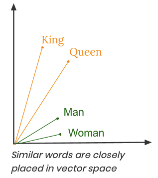
They have learned representations of text in an n-dimensional space where words that have the same meaning have a similar representation. Meaning that two similar words are represented by almost similar vectors that are very closely placed in a vector space.
For example, look at the below diagram, the words King and Queen appear closer to each other. Similarly the words Man and Woman appears closer to each other due to the kind of numeric vectors assigned to these words by GloVe. If you compute the distance between two words using their numeric vectors, then those words which are related to each other with a context, will have less distance between them.
So how these numeric vectors are generated for each word? Based on Co-occurence matrix.
Context Window
Similar words tend to occur together and will have similar context for example – Apple is a fruit. Mango is a fruit. Apple and mango tend to have a similar context i.e fruit.
Co-occurrence – For a given corpus, the co-occurrence of a pair of words say w1 and w2 is the number of times they have appeared together in a Context Window.
Context Window – Context window is specified by a number and the direction. Basically, how many words before and after a given word should be considered? So what does a context window of 2 (around) means? Let us see an example below

Co-occurence matrix
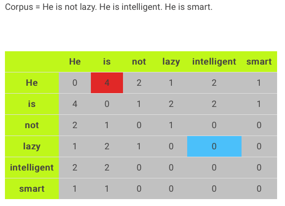
To understand the co-occurence matrix, consider the simple sentence below and the co-occurence matrix formed using a context window of 2 words.

Let’s say there are 5000 unique words in the corpus. So Vocabulary size = 5000. A co-occurrence matrix of size 5000 X 5000 will be formed.
Now, for even a decent corpus the size of all the unique words can easily get very large and difficult to handle. Imagine 1000000’s of words!!. So generally, this architecture is never preferred in practice.
Hence, instead of using the full 5000 X 5000 Co-occurrence matrix it is decomposed using techniques like PCA, SVD etc. into factors and combination of these factors forms the word vector representation.
For example, you perform PCA on this matrix of size 5000 X 5000. You will obtain 5000 principal components. Let’s say you selected 300 components out of these 5000 components. So, the new matrix will be of the form 5000 X 300.

Hence, a single word, instead of being represented in 5000 numbers will be represented in 300 numbers while still capturing almost the same semantic meaning.
This 300 number can vary from model to model.
Case Study: Support Ticket Classification using Glove
In a previous case study I showed you how can you convert Text data into numeric using TF-IDF. And then use it to create a classification model to predict the priority of support tickets.
In this case study I will use the same dataset and show you how can you use the numeric representations of words from Glove and create a classification model.
Problem Statement: Use the Microsoft support ticket text description to classify a new ticket into P1/P2/P3.
You can download the data required for this case study here.
Reading the support ticket data
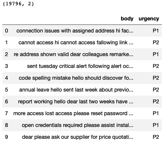
This data contains 19,796 rows and 2 columns. The column”body” represents the ticket description and the column “urgency” represents the Priority.
|
1 2 3 4 5 6 7 8 9 10 11 12 13 |
import pandas as pd import numpy as np import warnings warnings.filterwarnings('ignore') # Reading the data TicketData=pd.read_csv('supportTicketData.csv') # Printing number of rows and columns print(TicketData.shape) # Printing sample rows TicketData.head(10) |
Visualising the distribution of the Target variable
Now we try to see if the Target variable has balanced distribution or not? Basically each priority type has enough number of rows to be learned.
If the data would have been imbalanced, for example very less number of rows for P1 category, then you need to balance the data using any of the popular techniques like over-sampling, under-sampling or SMOTE.
|
1 2 3 4 5 6 7 |
# Number of unique values for urgency column # You can see there are 3 ticket types print(TicketData.groupby('urgency').size()) # Plotting the bar chart %matplotlib inline TicketData.groupby('urgency').size().plot(kind='bar'); |

The above bar plot shows that there are enough rows for each ticket type. Hence, this is balanced data for classification.
Count Vectorization: converting text data to numeric
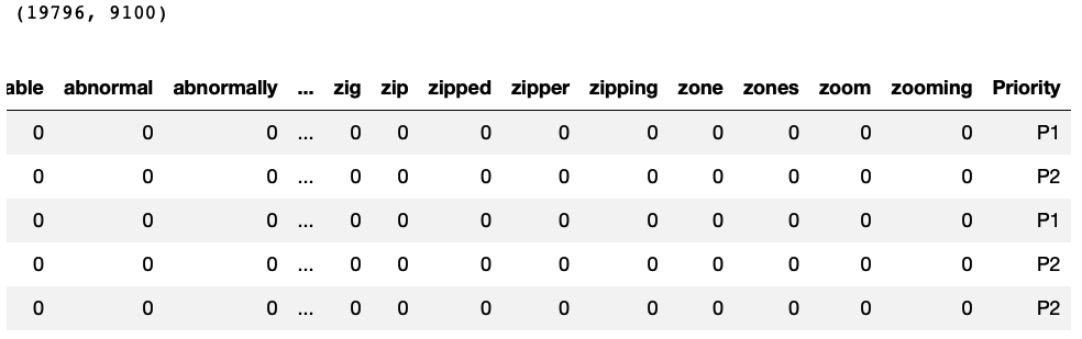
This step will help to remove all the stopwords and create a document term matrix.
We will use this matrix to do further processing. For each word in the document term matrix, we will use the GloVe numeric vector representation.
|
1 2 3 4 5 6 7 8 9 10 11 12 13 14 15 16 17 18 19 20 |
# Count vectorization of text from sklearn.feature_extraction.text import CountVectorizer # Ticket Data corpus = TicketData['body'].values # Creating the vectorizer vectorizer = CountVectorizer(stop_words='english') # Converting the text to numeric data X = vectorizer.fit_transform(corpus) #print(vectorizer.get_feature_names()) # Preparing Data frame For machine learning # Priority column acts as a target variable and other columns as predictors CountVectorizedData=pd.DataFrame(X.toarray(), columns=vectorizer.get_feature_names()) CountVectorizedData['Priority']=TicketData['urgency'] print(CountVectorizedData.shape) CountVectorizedData.head() |
GloVe conversion:
More information and model download: https://nlp.stanford.edu/projects/glove/
Please download “glove.6B.zip” from the above link, that is the GloVe model trained on 6Billion text tokens. All other files are >5GB and will probably hang your laptop!
Now we will use the GloVe representation of words to convert the above document term matrix to a smaller matrix, where the columns are the sum of the vectors for each word present in the document.
For example, look at the below diagram. The flow is shown for one sentence, the same happens for every sentence in the corpus.
- The numeric representation of each word is taken from GloVe.
- All the vectors are added, hence producing a single vector
- That single vector represents the information of the sentence, hence treated as one row.

Note: If you feel that your laptop is hanging due to the processing required for the below commands, you can use google colab notebooks!
From the glove.6B.zip folder I am choosing the version of glove which represents each word with 50-numbers.
|
1 2 3 4 5 6 7 8 9 10 |
# Defining an empty dictionary to store the values GloveWordVectors = {} # Reading Glove Data with open("/Users/farukh/Downloads/glove/glove.6B.50d.txt", 'r', encoding="utf-8") as f: for line in f: values = line.split() word = values[0] vector = np.array(values[1:], "float") GloveWordVectors[word] = vector |
|
1 2 |
# Checking the total number of words present len(GloveWordVectors.keys()) |

|
1 2 |
# Each word has a numeric representation of 50 numbers GloveWordVectors['bye'].shape |

|
1 2 |
# Sample glove word vector GloveWordVectors['bye'] |

|
1 2 3 4 5 |
# Creating the list of words which are present in the Document term matrix WordsVocab=CountVectorizedData.columns[:-1] # Printing sample words WordsVocab[0:10] |

Converting every sentence to a numeric vector
For each word in a sentence we extract the numeric form of the word and then simply add all the numeric forms for that sentence to represent the sentence.
|
1 2 3 4 5 6 7 8 9 10 11 12 13 14 15 16 17 18 19 20 21 22 23 24 |
# Defining a function which takes text input and returns one vector for each sentence def FunctionText2Vec(inpTextData): # Converting the text to numeric data X = vectorizer.transform(inpTextData) CountVecData=pd.DataFrame(X.toarray(), columns=vectorizer.get_feature_names()) # Creating empty dataframe to hold sentences W2Vec_Data=pd.DataFrame() # Looping through each row for the data for i in range(CountVecData.shape[0]): # initiating a sentence with all zeros Sentence = np.zeros(50) # Looping thru each word in the sentence and if its present in # the Glove model then storing its vector for word in WordsVocab[CountVecData.iloc[i, : ]>=1]: #print(word) if word in GloveWordVectors.keys(): Sentence=Sentence+GloveWordVectors[word] # Appending the sentence to the dataframe W2Vec_Data=W2Vec_Data.append(pd.DataFrame([Sentence])) return(W2Vec_Data) |
|
1 2 3 4 5 6 |
# Since there are so many words... This will take some time :( # Calling the function to convert all the text data to Glove Vectors W2Vec_Data=FunctionText2Vec(TicketData['body']) # Checking the new representation for sentences W2Vec_Data.shape |

|
1 2 |
# Comparing the above with the document term matrix CountVectorizedData.shape |

Preparing Data for ML
|
1 2 3 4 5 6 7 |
# Adding the target variable W2Vec_Data.reset_index(inplace=True, drop=True) W2Vec_Data['Priority']=CountVectorizedData['Priority'] # Assigning to DataForML variable DataForML=W2Vec_Data DataForML.head() |

Splitting the data into training and testing
|
1 2 3 4 5 6 7 8 9 10 11 12 13 14 15 16 |
# Separate Target Variable and Predictor Variables TargetVariable=DataForML.columns[-1] Predictors=DataForML.columns[:-1] X=DataForML[Predictors].values y=DataForML[TargetVariable].values # Split the data into training and testing set from sklearn.model_selection import train_test_split X_train, X_test, y_train, y_test = train_test_split(X, y, test_size=0.3, random_state=428) # Sanity check for the sampled data print(X_train.shape) print(y_train.shape) print(X_test.shape) print(y_test.shape) |

Standardization/Normalization
This is an optional step. It can speed up the processing of the model training.
|
1 2 3 4 5 6 7 8 9 10 11 12 13 14 15 16 17 18 19 20 21 22 23 |
from sklearn.preprocessing import StandardScaler, MinMaxScaler # Choose either standardization or Normalization # On this data Min Max Normalization is used because we need to fit Naive Bayes # Choose between standardization and MinMAx normalization #PredictorScaler=StandardScaler() PredictorScaler=MinMaxScaler() # Storing the fit object for later reference PredictorScalerFit=PredictorScaler.fit(X) # Generating the standardized values of X X=PredictorScalerFit.transform(X) # Split the data into training and testing set from sklearn.model_selection import train_test_split X_train, X_test, y_train, y_test = train_test_split(X, y, test_size=0.3, random_state=428) # Sanity check for the sampled data print(X_train.shape) print(y_train.shape) print(X_test.shape) print(y_test.shape) |
Training ML classification models
Now the data is ready for machine learning. There are 50-predictors and one target variable. We will use below algorithms and select the best one out of them based on the accuracy scores you can add more algorithms to this list as per your preferences.
- Naive Bayes
- KNN
- Logistic Regression
- Decision Trees
- AdaBoost
Naive Bayes
This algorithm trains very fast! The accuracy may not be very high always but the speed is guaranteed!
I have commented the cross validation section just to save computing time. You can uncomment and execute those commands as well.
|
1 2 3 4 5 6 7 8 9 10 11 12 13 14 15 16 17 18 19 20 21 22 23 24 25 26 27 28 29 30 31 |
# Naive Bayes from sklearn.naive_bayes import GaussianNB, MultinomialNB # GaussianNB is used in Binomial Classification # MultinomialNB is used in multi-class classification #clf = GaussianNB() clf = MultinomialNB() # Printing all the parameters of Naive Bayes print(clf) NB=clf.fit(X_train,y_train) prediction=NB.predict(X_test) # Measuring accuracy on Testing Data from sklearn import metrics print(metrics.classification_report(y_test, prediction)) print(metrics.confusion_matrix(y_test, prediction)) # Printing the Overall Accuracy of the model F1_Score=metrics.f1_score(y_test, prediction, average='weighted') print('Accuracy of the model on Testing Sample Data:', round(F1_Score,2)) # Importing cross validation function from sklearn from sklearn.model_selection import cross_val_score # Running 10-Fold Cross validation on a given algorithm # Passing full data X and y because the K-fold will split the data and automatically choose train/test Accuracy_Values=cross_val_score(NB, X , y, cv=5, scoring='f1_weighted') print('\nAccuracy values for 5-fold Cross Validation:\n',Accuracy_Values) print('\nFinal Average Accuracy of the model:', round(Accuracy_Values.mean(),2)) |

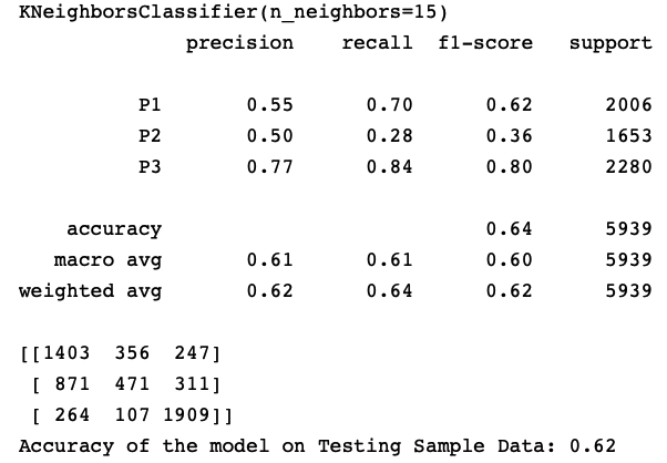
KNN
This is a distance based supervised ML algorithm. Make sure you standardize/normalize the data before using this algorithm, otherwise the accuracy will be low.
|
1 2 3 4 5 6 7 8 9 10 11 12 13 14 15 16 17 18 19 20 21 22 23 24 25 26 27 28 29 30 31 |
# K-Nearest Neighbor(KNN) from sklearn.neighbors import KNeighborsClassifier clf = KNeighborsClassifier(n_neighbors=15) # Printing all the parameters of KNN print(clf) # Creating the model on Training Data KNN=clf.fit(X_train,y_train) prediction=KNN.predict(X_test) # Measuring accuracy on Testing Data from sklearn import metrics print(metrics.classification_report(y_test, prediction)) print(metrics.confusion_matrix(y_test, prediction)) # Printing the Overall Accuracy of the model F1_Score=metrics.f1_score(y_test, prediction, average='weighted') print('Accuracy of the model on Testing Sample Data:', round(F1_Score,2)) # Importing cross validation function from sklearn from sklearn.model_selection import cross_val_score # Running 10-Fold Cross validation on a given algorithm # Passing full data X and y because the K-fold will split the data and automatically choose train/test #Accuracy_Values=cross_val_score(KNN, X , y, cv=10, scoring='f1_weighted') #print('\nAccuracy values for 10-fold Cross Validation:\n',Accuracy_Values) #print('\nFinal Average Accuracy of the model:', round(Accuracy_Values.mean(),2)) # Plotting the feature importance for Top 10 most important columns # There is no built-in method to get feature importance in KNN |
Logistic Regression
This algorithm also trains very fast. Hence, whenever we are using high dimensional data, trying out Logistic regression is sensible. The accuracy may not be always the best.
|
1 2 3 4 5 6 7 8 9 10 11 12 13 14 15 16 17 18 19 20 21 22 23 24 25 26 27 28 29 30 31 32 33 34 35 36 37 38 |
# Logistic Regression from sklearn.linear_model import LogisticRegression # choose parameter Penalty='l1' or C=1 # choose different values for solver 'newton-cg', 'lbfgs', 'liblinear', 'sag', 'saga' clf = LogisticRegression(C=10,penalty='l2', solver='newton-cg') # Printing all the parameters of logistic regression # print(clf) # Creating the model on Training Data LOG=clf.fit(X_train,y_train) # Generating predictions on testing data prediction=LOG.predict(X_test) # Printing sample values of prediction in Testing data TestingData=pd.DataFrame(data=X_test, columns=Predictors) TestingData['Survived']=y_test TestingData['Predicted_Survived']=prediction print(TestingData.head()) # Measuring accuracy on Testing Data from sklearn import metrics print(metrics.classification_report(y_test, prediction)) print(metrics.confusion_matrix(prediction, y_test)) ## Printing the Overall Accuracy of the model F1_Score=metrics.f1_score(y_test, prediction, average='weighted') print('Accuracy of the model on Testing Sample Data:', round(F1_Score,2)) ## Importing cross validation function from sklearn #from sklearn.model_selection import cross_val_score ## Running 10-Fold Cross validation on a given algorithm ## Passing full data X and y because the K-fold will split the data and automatically choose train/test #Accuracy_Values=cross_val_score(LOG, X , y, cv=10, scoring='f1_weighted') #print('\nAccuracy values for 10-fold Cross Validation:\n',Accuracy_Values) #print('\nFinal Average Accuracy of the model:', round(Accuracy_Values.mean(),2)) |

Decision Tree
This algorithm trains slower as compared to Naive Bayes or Logistic, but it can produce better results.
|
1 2 3 4 5 6 7 8 9 10 11 12 13 14 15 16 17 18 19 20 21 22 23 24 25 26 27 28 29 30 31 32 33 34 |
# Decision Trees from sklearn import tree #choose from different tunable hyper parameters clf = tree.DecisionTreeClassifier(max_depth=20,criterion='gini') # Printing all the parameters of Decision Trees print(clf) # Creating the model on Training Data DTree=clf.fit(X_train,y_train) prediction=DTree.predict(X_test) # Measuring accuracy on Testing Data from sklearn import metrics print(metrics.classification_report(y_test, prediction)) print(metrics.confusion_matrix(y_test, prediction)) # Printing the Overall Accuracy of the model F1_Score=metrics.f1_score(y_test, prediction, average='weighted') print('Accuracy of the model on Testing Sample Data:', round(F1_Score,2)) # Plotting the feature importance for Top 10 most important columns %matplotlib inline feature_importances = pd.Series(DTree.feature_importances_, index=Predictors) feature_importances.nlargest(10).plot(kind='barh') # Importing cross validation function from sklearn #from sklearn.model_selection import cross_val_score # Running 10-Fold Cross validation on a given algorithm # Passing full data X and y because the K-fold will split the data and automatically choose train/test #Accuracy_Values=cross_val_score(DTree, X , y, cv=10, scoring='f1_weighted') #print('\nAccuracy values for 10-fold Cross Validation:\n',Accuracy_Values) #print('\nFinal Average Accuracy of the model:', round(Accuracy_Values.mean(),2)) |

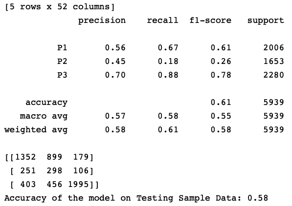
Adaboost
This is a tree based boosting algorithm. If the data is not high dimensional, we can use this algorithm. otherwise it takes lot of time to train.
|
1 2 3 4 5 6 7 8 9 10 11 12 13 14 15 16 17 18 19 20 21 22 23 24 25 26 27 28 29 30 31 32 33 34 35 36 37 |
# Adaboost from sklearn.ensemble import AdaBoostClassifier from sklearn.tree import DecisionTreeClassifier # Choosing Decision Tree with 1 level as the weak learner DTC=DecisionTreeClassifier(max_depth=2) clf = AdaBoostClassifier(n_estimators=20, base_estimator=DTC ,learning_rate=0.01) # Printing all the parameters of Adaboost print(clf) # Creating the model on Training Data AB=clf.fit(X_train,y_train) prediction=AB.predict(X_test) # Measuring accuracy on Testing Data from sklearn import metrics print(metrics.classification_report(y_test, prediction)) print(metrics.confusion_matrix(y_test, prediction)) # Printing the Overall Accuracy of the model F1_Score=metrics.f1_score(y_test, prediction, average='weighted') print('Accuracy of the model on Testing Sample Data:', round(F1_Score,2)) # Importing cross validation function from sklearn #from sklearn.model_selection import cross_val_score # Running 10-Fold Cross validation on a given algorithm # Passing full data X and y because the K-fold will split the data and automatically choose train/test #Accuracy_Values=cross_val_score(AB, X , y, cv=10, scoring='f1_weighted') #print('\nAccuracy values for 10-fold Cross Validation:\n',Accuracy_Values) #print('\nFinal Average Accuracy of the model:', round(Accuracy_Values.mean(),2)) # Plotting the feature importance for Top 10 most important columns #%matplotlib inline #feature_importances = pd.Series(AB.feature_importances_, index=Predictors) #feature_importances.nlargest(10).plot(kind='barh') |

Training the best model on full data
KNN algorithm is producing the highest accuracy on this data, hence selecting it as final model for deployment.
|
1 2 3 4 |
# Generating the KNN model on full data # This is the best performing model clf = KNeighborsClassifier(n_neighbors=15) FinalModel=clf.fit(X,y) |
Making predictions on new cases
To deploy this model, all we need to do is write a function which takes the new data as input, performs all the pre-processing required and passes the data to the Final model.
|
1 2 3 4 5 6 7 8 9 10 11 12 13 14 15 16 17 |
# Defining a function which converts words into numeric vectors for prediction def FunctionPredictUrgency(inpText): # Generating the Glove word vector embeddings X=FunctionText2Vec(inpText) #print(X) # If standardization/normalization was done on training # then the above X must also be converted to same platform # Generating the normalized values of X X=PredictorScalerFit.transform(X) # Generating the prediction using Naive Bayes model and returning Prediction=FinalModel.predict(X) Result=pd.DataFrame(data=inpText, columns=['Text']) Result['Prediction']=Prediction return(Result) |
|
1 2 3 |
# Calling the function NewTicket=["please help to review", "Please help to resolve system issue"] FunctionPredictUrgency(inpText=NewTicket) |

Conclusion
Transfer learning has made NLP research faster by providing an easy way to share the models produced by big companies and build on top of that. Similar to GloVe we have other algorithms like Word2Vec, Doc2Vec and BERT which I have discussed in separate case studies.
I hope this post helped you to understand how GloVe vectors are created and how to use them to convert any text into numeric form.
Consider sharing this post with your friends to spread the knowledge and help me grow as well! 🙂