Principal Component Analysis(PCA) is an unsupervised machine learning algorithm that is used for dimension reduction in data. Basically, it is a way to represent the information of many columns with only a few columns known as the principal components.
More information about this algorithm can be found here and in the below video.
The below code snippet helps to find principal components of a given data.
|
1 2 3 4 5 6 7 8 9 10 11 12 13 14 15 16 17 18 19 20 21 22 23 24 25 26 27 28 29 30 31 32 33 34 35 36 37 38 39 40 41 42 43 44 45 46 47 48 |
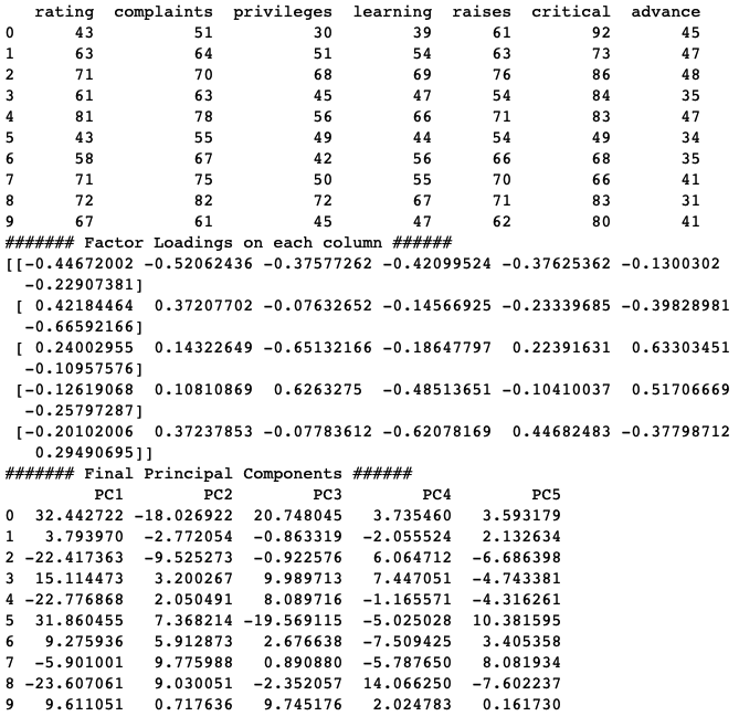
# Sample code to do PCA in Python # Creating the employee attitude survey data for PCA rating=[43,63,71,61,81,43,58,71,72,67,64,67,69,68,77,81,74,65,65,50,50,64,53,40,63,66,78,48,85,82] complaints=[51,64,70,63,78,55,67,75,82,61,53,60,62,83,77,90,85,60,70,58,40,61,66,37,54,77,75,57,85,82] privileges=[30,51,68,45,56,49,42,50,72,45,53,47,57,83,54,50,64,65,46,68,33,52,52,42,42,66,58,44,71,39] learning=[39,54,69,47,66,44,56,55,67,47,58,39,42,45,72,72,69,75,57,54,34,62,50,58,48,63,74,45,71,59] raises=[61,63,76,54,71,54,66,70,71,62,58,59,55,59,79,60,79,55,75,64,43,66,63,50,66,88,80,51,77,64] critical=[92,73,86,84,83,49,68,66,83,80,67,74,63,77,77,54,79,80,85,78,64,80,80,57,75,76,78,83,74,78] advance=[45,47,48,35,47,34,35,41,31,41,34,41,25,35,46,36,63,60,46,52,33,41,37,49,33,72,49,38,55,39] #Joining all the vectors together to form input matrix X SurveyData=list(zip(rating,complaints,privileges,learning,raises,critical,advance)) import pandas as pd InpData=pd.DataFrame(data=SurveyData, columns=["rating","complaints","privileges","learning","raises","critical","advance"]) print(InpData.head(10)) #Creating input data numpy array X=InpData.values ###################################################################### # Creating maximum number of principal components from sklearn.decomposition import PCA pca = PCA(n_components=X.shape[1]) PrincipalComponents=pca.fit(X) # Finding the variance explained by each component import numpy as np var_explained= PrincipalComponents.explained_variance_ratio_ var_explained_cumulative=np.cumsum(np.round(var_explained, decimals=4)*100) # plotting the variance explained to find optimal number of components plt.plot(np.array(range(1,8)),var_explained_cumulative) # By Looking at below graph we can see that 5 components are explaining maximum Variance # in the dataset the elbow/saturation occurs at 5th principal component # choosing 5 principal components based on above graph pca = PCA(n_components=5) FinalPrincipalComponents = pca.fit_transform(X) # Understanding the loadings print('####### Factor Loadings on each column ######') loadings = pca.components_ print(loadings) # Creating the Principal Component data FinalPC=pd.DataFrame(FinalPrincipalComponents, columns=['PC1','PC2','PC3','PC4','PC5']) print('####### Final Principal Components ######') print(FinalPC.head(10)) |
Sample Output

Author Details
Lead Data Scientist
Farukh is an innovator in solving industry problems using Artificial intelligence. His expertise is backed with 10 years of industry experience. Being a senior data scientist he is responsible for designing the AI/ML solution to provide maximum gains for the clients. As a thought leader, his focus is on solving the key business problems of the CPG Industry. He has worked across different domains like Telecom, Insurance, and Logistics. He has worked with global tech leaders including Infosys, IBM, and Persistent systems. His passion to teach inspired him to create this website!