
In the previous post, I talked about the data science interview questions from reinforcement learning. In this post, I am going to talk about supervised Deep Learning algorithms which are helping us to create a lot of modern applications based on AI. For example, Alexa, Siri, face recognition in our mobile phone cameras, scene detection in our phone cameras, language translation in Google, etc. the list is long!
And what made all of this possible? The idea of a tiny artificial neuron! Which evolved to Artificial Neuron Networks(ANN), Convolutional Neuron Networks(CNN), Recurrent Neural Networks(RNN), Long Short Term Memory Networks(LSTM), etc. I will explain each of these in-depth in this article. Let us begin!
Table of contents
- What is Deep Learning?
- What are the types of Deep Learning?
- What is an Artificial Neuron?
- What happens inside a Neuron?
- What happens inside a transfer function?
- What happens inside an activation function?
- How does an Artificial Neuron learn?
- What are the different types of activation functions?
- What is an Artificial Neural Network(ANN)?
- What is the Input layer inside an ANN?
- What is the Hidden layer inside an ANN?
- What is the Output layer inside an ANN?
- How does an Artificial Neural Network(ANN) learn?
- What is a Convolutional Neural Network(CNN)?
- What happens during the Convolution step inside CNN?
- What happens during the Max-Pooling step inside CNN?
- What happens during the Flattening step inside CNN?
- What is a Recurrent Neural-Network(RNN)?
- What is Back Propagation Through Time (BPTT)?
- What are Seq2Seq models?
- What is a Long Short Term Memory Network(LSTM)?
- What is the problem of Vanishing Gradient?
- What is the difference between RNN and LSTM?
- What are the practical applications of ANN?
- What are the practical applications of CNN?
- What are the practical applications of RNN and LSTM?
Q. What is Deep Learning?
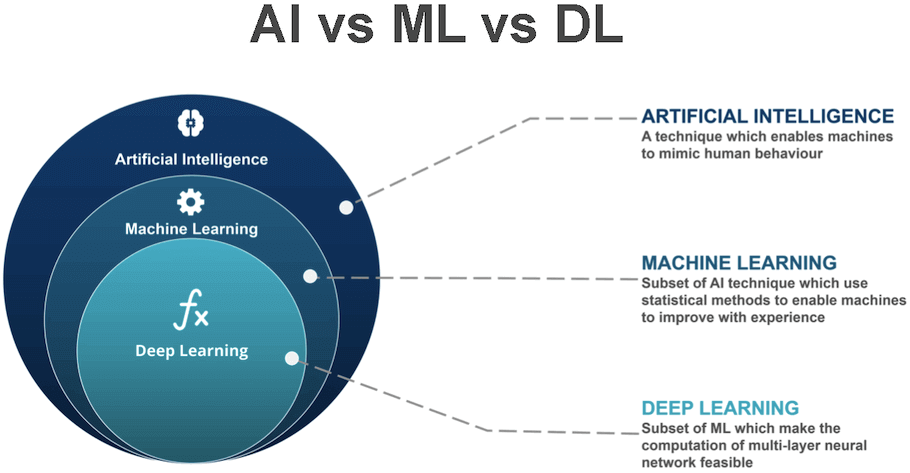
Deep learning is a part of machine learning, which is in turn part of a larger umbrella called AI.
In other words, you can say Deep Learning is a special type of machine learning consisting of few algorithms which are designed to learn from large amounts of data or unstructured data like images, texts, and audio. These algorithms are inspired by the way our brain works. Deep learning algorithms like ANN, CNN, RNN, LSTM, etc. attempt to mimic the behavior of the neural network present in our brains!
Q. What are the types of Deep Learning?
There are two major types of deep learning, supervised and unsupervised.
Supervised Deep Learning: Those algorithms which are trained by input and output examples. Just like supervised machine learning algorithms, we create an input matrix (X) having predictors and output matrix (y) having the target variable. We pass this data to the algorithms to learn. Most notable algorithms from supervised deep learning are listed below.
- Artificial Neural Networks(ANN)
- Convolutional Neural Networks(CNN)
- Recurrent Neural Networks(RNN)
- Long Short Term Memory Networks(LSTM)
Unsupervised Deep Learning: Those algorithms where we pass the whole data as input. There is no target variable, hence, we derive the patterns out the data directly without any supervision or explicit training. Just like unsupervised machine learning. Most notable algorithms from unsupervised deep learning are listed below.
- Self Organising Maps (SOM)
- Restricted Boltzmann machines(RBM)
- Autoencoders
- Deep Belief Networks(DBN)
Q. What is an Artificial Neuron?
An artificial neuron is a way to mimic the biological neuron, which is the building block of the human brain. If you want to understand all the algorithms of Deep Learning, then understanding how an artificial neuron work is very critical.

The basic working idea of a biological neuron is that they transfer electrical impulses to other neurons, there are billions of neurons interconnected together inside our brain, and which are in turn connected to the spinal cord spreading nerves throughout the body collectively called the nervous system.
So when we touch/feel/sense/smell/see anything, the receptors send information to the spinal cord and spinal cord sends the signal to our brain, and certain parts of our brain get activated because there are multiple neurons in that part that got “activated” and starts sending electrical impulses in that area known as neurons “firing“.
Hence, when we touch something, that neurons belonging to that light blue area(Parietal Lobe) gets activated. In other words, when the electrical impulses of that area exceed a certain threshold, we say the neurons are “activated“.

But…why does a neuron gets activated?
A neuron gets activated due to the kind of input signal received from the spinal cord which will increase the chemical inside the neuron more than a threshold, hence making the neuron to “fire” and send the signal to the other connected neurons.
Let’s understand how this knowledge is used to create an Artificial Neuron.
Consider the tiny data shown below which shows when a loan got approved or not based on the salary of the applicant and the CIBIL score. If we need to show this data to a neuron then the output(y) will be the loan_status column and the inputs will be Salary(X1) and CIBIL(X2) and Amount(X3) columns.

The inputs(X1, X2, and X3) will be passed to the input neurons, if there were 10 inputs then we will use 10 input neurons to accept all the values. I have shown it for one row, similarly, it happens for all the rows in the data.

What Happens inside a Neuron?
- Step–1: Inputs are passed as inputs to the Artificial Neuron which are multiplied by weights and a bias is added to them inside the transfer function.
- Step–2: Then the resultant value is passed to the activation function. The result of the activation function is treated as the output of the neuron.
What “Transfer function” does?
The transfer function creates a weighted sum of all the inputs and adds a constant to it called bias.
W1*X1 + W2*X2 + W3*X3 . . . Wn*Xn + b
Here W1, W2, W3, etc. are weights randomly initialized for X1 and X2. Here in the above example that calculation is W1*30000 + W2*350 + W3*750000 +b
And what “Action function” does?
The activation function takes the input from the Transfer function and produces an outcome based on it. There are various activation functions in use today. Some of the popular ones are the Step Function, the Sigmoid Function, the ReLu function, and the tanh function. depending upon the function equation, some of these produce output in the range of 0 to 1, some of them between -1 to 1 and some of them between -inf to +inf. We will discuss more about these in the next section.
Q. How does an Artificial Neuron learn?
Consider the same tiny data for loan approval shown above.
We would want that out Artificial Neuron could learn when to approve a loan or not based on the examples we show to it.
For that, we “train” the neuron by showing each of these examples one by one and asking the neuron to “adjust” all those weights W1, W2, W3, etc. and the bias such that, it can explain the whole data.
To perform this, the below steps takes place after the input data is passed to the neuron.
- Each input value is multiplied with a small number (close to zero) called Weights
- All of these values are summed up
- A number is added to this sum called Bias
- The above summation is passed to a function called “Activation Function“
- The Activation function will produce an output based on its equation. Sometimes this will range between (0 to 1) e.g. ReLu and sometimes between (-1 to 1) e.g. Sigmoid.
- The output produced will be sent as an input to the other neuron so on and so forth.
- The output produced by the neurons in the last layer of the network is treated as the output.
- If the output produced by the neurons does not match with the actual answer, then the error signals are sent back in the network which adjusts the weights and the bias values such that the output comes closer to the actual value this process is known as Backpropagation.
- The steps 1-8 are repeated again till the difference between the actual value and the predicted value(output of the neuron) becomes equal or almost equal and there is no further improvement happening… this situation is known as convergence. When we say the algorithm has reached its maximum possible accuracy.
Q. What are the different types of activation functions?
There are many activation functions, they differ from each other mainly based on the kind of output they produce once the weighted sum from transfer function is passed to it.
Each activation function has its own equation, which defines how it works and the kind of output it produces. Some of the most popular activation functions are Threshold, Linear, Sigmoid, TanH, and ReLU
Their equations and diagrams are shown below. The X-Axis represents the net sum received from the transfer function, which is the weighted average of the inputs. The Y-Axis represents the output of the function based on the values of the input.

Let me explain Relu and Sigmoid as these are the two most widely used activation functions
ReLu and Sigmoid activation functions are most widely used for Neural Networks
If the input value to the Relu function is less than zero, then the output is zero, but if the value is greater than zero, then the output is equal to whatever the input is. This is by far the most widely used activation function.
If the input value to Sigmoid is negative, then it produces output values close to 0 and if the input value is positive then it produces the output values close to 1. The sigmoid function is very handy when we are creating binary classification Neural Network models.
Q. What is an Artificial Neural Network(ANN)?
When we combine multiple neurons together, it creates a vector of neurons called a layer.
When we combine multiple layers together, where all the neurons are interconnected to each other, this network of neurons is called, Artificial Neural Network or abbreviated as ANN


There are three major type of layers in the ANN listed below
- The Input layer (interface to accept data)
- The Hidden layer(s) (Actual Neurons)
- The Output layer (Actual Neurons to output the result)
The Input Layer
There is only one Input layer, which takes the data input and passes it to the network. Mind that this layer is simply the data vector which is passed. It does not comprise of an actual neuron layer, it is just an interface to accept data for the hidden layers, which are the actual neurons.
Thinking of the input layer as neurons is the most common misunderstanding which leads to confusion later on while implementing the code! Please keep this in mind!
The input layer shown in all the ANN diagrams are NOT neurons, they are just interfaces to accept the data.
The Hidden Layer(s)
There could be one or more hidden layers in a given ANN. These are the actual neurons that perform the calculations on the input data.
How many hidden layers should be used? There is no definitive answer to that question. Determining the optimal number of hidden layers and how many neurons will be present in each layer is a huge challenge and it is done by observing the final accuracy for various combinations.
The Output Layer
There is only one output layer and the number of neurons in it depends on the target variable. Most common settings are listed below
- Regression: One single Neuron in the output layer generating the continuous number predictions
- Binary Classification: One single Neuron generating either 1 or 0 indicating the classes
- Multi-Class Classification: Multiple Neurons equal to the number of classes each representing the output for one class
Q. How does an Artificial Neural Network(ANN) learn?
I have briefly discussed this answer above, let’s dig deeper into it.
The Artificial Neural Network learns by multiple iterations of forward propagation and backward propagation.

- Forward Propagation: Transferring information from the input layer to the output layer
- Back Propagation: Transferring error information from the output layer to the hidden layers and adjusting weights of each hidden layer.
Throughout the iterations, the ANN keeps comparing the actual output with the predicted output and adjusts all the weights in the network to make the predicted values equal to the actual values.
ANN keeps comparing the actual output with the predicted output and adjusts all the weights in the network to make the predicted values equal to the actual values.
The first step is to multiply all the inputs(X1, X2, X3…etc) with a random weight(W1, W2, W3…etc). These random values are decided by an algorithm called kernel_initializer in the Keras library. These random values are initialized as very small numbers(non-zero). Each neuron has its own set of weights.
Now, these weighted inputs are passed to the transfer function of each of the neutrons. The transfer function sums the weighted inputs and adds another constant value to it called bias. Initially, Bias(b) is also a small non-zero number. This step forms an equation shown below
Net Sum=W1*X1 + W2*X2 + W3*X3 . . . Wn*Xn + b
The Net Sum found above by the transfer function is sent to the activation function as input. The output generated by the activation function is the output of the Neuron. Each neuron produces its output which is passed as input to the neutrons in the next layer. The output of neurons in the last layer called the output layer is treated as the final output of the ANN.
Neuron Output = Activation Function( Net Sum )
The Neuron Output is compared with the actual value, and error(loss) is computed depending on the type of problem statement as listed below
- Regression Loss: Mean Squared Error, Mean Squared Logarithmic Error, Mean Absolute Error
- Binary Classification: Binary Cross-Entropy, Hinge, Squared Hinge
- Multi-Class Classification: Multi-Class Cross-Entropy, Sparse Multiclass Cross-Entropy, Kullback Leibler Divergence
The goal of ANN is to generate as minimum loss as possible. Ideal value would be zero, but, we never see zero loss practically. At best it would be a very small number like 0.0000000023.
With this, one round of Forward Propagation is finished.
Now the ANN will start adjusting the weights and bias values for each of the layers starting from the output layer to each one of the hidden layers one by one in the backward direction. The goal to reduce the loss value which in turn will reduce the difference between the predicted value and the original value.
This adjustment of weights is done based on the direction(Gradient) of the loss and since we are trying to reduce the loss, we always choose such weights which will generate lower loss values and the “direction” of movement of loss is downwards, hence, this technique is known as Gradient Descent.
When the weight of all the hidden layers is adjusted, we say one round of Back Propagation is finished.
During one cycle of forward propagation and backpropagation, ANN learns only one single row from the data. This cycle is repeated for every row in the data. When all the rows are finished, we call it one single epoch.
Does the network adjust the weights for each and every row all the time?
When the ANN updates the weights after learning one single row, it is known as Stochastic Gradient Descent (SGD). Here the gradient of the error is calculated using the error of only one row in data. Hence, weights are updated for every round of forward and backward propagations. When all the rows are completed. we call it one epoch.
On the other extreme when the ANN updates the weights only after learning ALL the rows in the data, it is known as Batch Gradient Descent (BGD). Here, the gradient of the error is calculated using the errors of ALL the rows in the data together. When all the rows are finished we call it one epoch.
An approach falling between the above two is known as Mini Batch Gradient Descent. Here the ANN updates the weight of the Network after learning a few rows in the data. We can decide how many rows shall we consider like 5 rows, 10 rows, 50 rows, etc. The gradient of the error is computed by using the errors of the specified number of rows at a time. When all the rows are finished batch by batch, we call it one epoch.
We perform multiple epochs to get the best possible weights. Which will provide the highest accuracy.
Q. What is a Convolutional Neural Network(CNN)?
Convolutional Neural Networks are special kind of Neural Networks which helps the machine to learn and classify the images. A good example is the Face Recognition.
Let’s say, you click click 50 pictures of a person’s face, and you click them for 10 persons. So in total, you have 500 pictures of 10 different persons. If you pass this data to CNN, it will learn how each of these 10 person’s face looks like. And, later on when you show a new picture of one of these 10 persons, then it will recognize the face based on the previous learnings.
CNN tries to mimic the way we humans look at the images through our eyes.
CNN tries to mimic the way we humans look at the images through our eyes. If you think about it, you will notice that you can focus only at one particular point at a time even when you are looking at a whole picture, and then we shift our focus to look at the other points and that’s how we learn a picture or a face, by memorizing the important characteristics.
CNN is a combination of steps which first derives the most import characteristics of a given image and then convert the whole image into a single row of numbers. Which can be learned by the fully connected ANN classifier.
Consider the below image of a dog. The way our computer stores this image is by using pixels. So CNN tries to identify the most important pixels which are unique to a dog which is the black pixels of his nose, mouth, and eyes, the pixels outlining the shape of the dog’s face, the pixels outlining the large ears of the dog… so on and so forth.
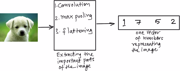
Hence, using steps like Convolution, Max pooling and, Flattening, CNN finds out the most important pixel combinations in the image and represents them as a set of numbers. Each of these numbers represents a unique feature of the image.

When you use multiple images then each image is represented by a row vector in the data, and it starts to look like any other supervised machine learning dataset. We will use a fully connected ANN on top of this data to learn all the images and their respective labels.
In case of face recognition, the labels will the names of the persons. In the case of animal recognition, it will be the names of each animal like a cat, dog, mouse, etc.

Summarizing the whole CNN flow with the below diagram. First, you extract the important features from the images, hence, converting the images into a set of numbers. These numbers are learned by the Artificial Neural Network against a label.

In the following section, we will discuss what happens inside Convolution, Max Pooling, and Flattening which extracts the most important features from the images.
Q. What happens during the Convolution step inside CNN?
Convolution is a unique idea that enables us to convert the unstructured image data into structured data.
In simple terms, we extract the most important pixels from the image and summarize the digital information of the image. For this, we use filters also known as kernels.
Imaging yourself analyzing an image very closely using a magnifying glass, you would be moving the magnifying glass slowly from left to right to observe each and every part of the image, in the process, you will notice every minute details and register those details in your brain. Filters/kernels try to mimic the same operation.
There are multiple types of filters, each filter will pick a different detail from the image based on its design. The size of a filter also varies, the most common size of the filter is (3X3) matrix, but it can be (4X4) or (5X4) also.
To understand the working of a filter/kernel, take a look at the below image. The image of the dog is represented by a digital matrix of numbers, now using the filter, we sweep through the digital matrix of image one filter block at a time, the filter block is looking at 9 pixels at a time. If we sweep by increasing one pixel then we say stride=1, if we sweep by moving two pixels at a time then we say stride=2.
The sweep operation is just the multiplication of original image numbers with the numbers inside the filter. The numbers inside the filter can change based on the type of filter.

Once the filter moves through the image, a summarised digital image is formed, as shown above, it is also called the feature map or the activation map because we have mapped or extracted the most important features from the original image using the filter.
Q. What happens during the Max-Pooling step inside CNN?
After the Convolution step, we perform one more step of extracting the most important feature from the image, this step helps to reduce the dimensionality of the image data, which in turn helps in fast computations during the ANN step at the end.
The concept is similar to Convolution, there is a Max-Pooling filter that is passed through the data and the maximum value in that filter is selected as the final feature. In the below diagram, you can see a Max-Pooling filter for the dimension (2X1) when passed through the feature map it selects the maximum value of each window as the final feature.

The size of the max-pool filter can also be flexible like the convolution filter. It can be (2X2), (3X3), (4X5), etc. The bigger the filter the more compressed the image information is. since it will sweep bigger areas and take the maximum value from those areas.
Q. What happens during the Flattening step inside CNN?
This is the final step in extracting the most important features from an image inside CNN. We just ‘unfold’ the max-pooled data and convert it into a vector, simply by arranging the numbers in one dimension.

After this, the data can be fed to a fully connected Dense layer and learn it against the labels.
Q. What is a Recurrent Neural Network(RNN)?

The human brain can retain information, short term, and long term both. We can look back in time to remember the chain of events that happened and guess what will happen next based on the previous chain of events. Recurrent Neural Networks(RNN) tries to mimic this ability.
Consider the scenario when you are reading a book, you understand the events of a chapter based on the events of previous chapters. In a way, you look back in your brain to reference the previous set of events that help you to understand the current events. Some events are from the previous chapter and some events are from two or three chapters before. All these events are stored in memory with a sense of time that this event happened recently, and that event happened a long time back.
You remember the recent events better than the events that happened a long time back as the recent events are “fresh” in your memory. Hence the recent events affect your understanding of the current event or help you to guess or “predict” what is going to happen next.
Let’s take a look at a very simple example to help you realize how effortlessly our brain does this! Tell me what is the next number in the sequence below
8, ?
Since you saw only one number, the most obvious/logical answer which comes to mind is “9”. Simply because 8 comes before 9 in the digits sequence. As you have seen/learned many many such sequences in your life, for example, 1–>2, 2–>3, 3–>4, 20–>21, etc.
This can be the most simple example for One to One RNN. Where you input one single number and the output is one single number.
Now, if I show you another sequence and ask you to tell me what is the next value your brain will process the event differently.
2, 4, 6, 8, ?
Now the answer which came to your mind was 10! instead of “9” which you answered above! because you observed the previous numbers and effortlessly made a sequence in your head that the next number is always two values more from the previous number because you saw below sequence in your mind.
2–>4 (Time=t)
4–>6 (Time=t+1)
6–>8 (Time=t+2)
8–>10 (Time=t+3)
This can be the most simple example for Many to One RNN. Where you input a sequence of numbers and the output is one single number.
Another round of the same activity! Tell me what will be the next sequence of values in the below example.
1, 1, 1, 1 –> 2, 2, 2, 2
2, 2, 2, 2 –> 4, 4, 4, 4
2, 2, 3, 4 –> 4, 4, 6, 8
3, 3, 1, 1 –> ?
Once again our brain quickly works and figures out a ‘relationship’ between the outputs and the inputs, mathematically we call this relationship a “function”. By looking at the given examples, you understood that every value in the output is twice the value in the input hence you answer 6, 6, 2, 2.
This could be the most simple example of Many To Many RNNS. Where you input a sequence of numbers and the output is also a sequence of numbers.
All this was possible because of your ability to look at the “past” sequences of values and learn from them.
RNN tries to do the same thing. It looks back in time at the events that happened and learns the relationship between output and input.
RNN tries to look back in time at the events that happened and learns the relationship between output and input.
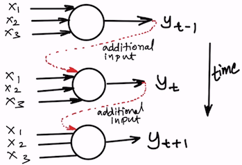
The special thing about RNN is that it looks back in time. That means it “knows” what has happened in the previous step. From the neural network architecture perspective, each neuron inside the hidden layer of an RNN knows the output the same neuron has produced in the previous “time step”. And, the output of the previous time step is used as an additional input for the current time step.
Each neuron inside the hidden layer of an RNN knows the output the same neuron has produced in the previous “time step”.
This means the whole neural network we created is virtually replicated multiple times based on how far away we need to look back in time. All the neurons in the hidden layer can look back at themselves and see what output they produced previously and use that to improve the output in the upcoming steps.
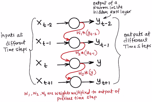
The below diagram will help to visualize the working of an RNN. You can see the whole RNN is repeated over time. The output of the hidden layers of the previous time step is fed to the same hidden layers in the next time step as shown below with red lines.

Back Propagation Through Time (BPTT).
Mathematically, when the network back propagates the errors, it does not just go back to the hidden layers, it also goes back to the hidden layers in the previous time steps. This activity is known as Back Propagation Through Time (BPTT). The weights of the network are adjusted based on the change in the error gradient through time as well. From the diagram above, the weights for the red lines are adjusted along with the black lines.
There are a number of modern applications that are based out of this concept of RNNs starting from sentiment analysis, image captioning, subtitle generation to chatbots.
Seq2Seq models
In general, when we combine two RNNs together where he first RNN accepts input as a sequence and the second RNN outputs a sequence we call it the Seq2Seq model.
Seq2Seq paves the path for many amazing applications. For example, Image summarization, Text Summarization, Image Captioning, Autocorrect, Language Translation, chatbots, etc. The basic idea for all these applications remains the same as listed below
- Generate lot of input and output sequences as examples to be learned
- Learn all the examples using Seq2Seq models
- Predict the output sequence for a new input sequence.
There are 4 types of Seq2Seq RNN models
- One to One: One number as input and one number as output. e.g Image classification
- One to Many: One number as input and many numbers as output. e.g Image captioning.
- Many to One: Many numbers as input and one number as output. e.g Sentiment analysis, Stock Price Prediction
- Many to Many: Many numbers as input and many numbers as output. e.g. Chatbots, Language Translation, auto email generation
Q. What is a Long Short Term Memory Network(LSTM)?
While RNNs are great, there is a problem with RNNs. The inability to store long term information. This improvisation to store and remember long term information is named as Long Short Term Memory Networks or LSTMs in short.
In order to understand why LSTM was invented. you need to first understand the problem with RNNs, which is known as the problem of Vanishing Gradient.
The problem of Vanishing Gradient
Every Deep Artificial Neural Network struggles with this problem. When the backpropagation begins at the output layer, it travels back towards the input layer while adjusting the weights of the each layer one by one based on the gradient of the cost function. In simple terms, the weights are adjusted so that the error is minimal at the output layer.
If the weight values are less than one. then the gradient will keep decreasing in the successive layer which will lead to no change in weights for faraway layers. The weights of last hidden layer are adjusted the most as it is closest to the output layer, the weights of the second last hidden layer are adjusted little less because it is away from the output layer, the more we go away from the output layer the lesser the weights are adjusted because of the diminishing gradient of the error. This issue, in general, is known as the problem of Vanishing gradient.
On the opposite end, if the weight values are greater than one, then the gradient will keep increasing in the successive layers during backpropagation, which will lead to big changes in the weights. This is known as the problem of Exploding gradient.
These problems become more pronounced in the RNNs as there we backpropagate through time as well. This leads to the inability of RNNs to remember long term information. This is where LSTMs kick in!
LSTMs solve this problem by introducing the concept of “memory cells“. The idea is to maintain a log of what is important and what is not through time. These memory cells store important information and reject non-important information. This enables LSTMs to “remember” important information and understand long term dependencies in data.
The idea behind LSTM memory cells is to maintain a log of what is important and what is not through time. These memory cells store important information and reject non-important information.
Look at the below image which describes the memory cells of the LSTM. It is like a link connecting all the time steps. The information is stored and deleted based on its importance. This memory cell information affects the output of the Neuron at each time step.

Hence, LSTMs are currently the most widely used algorithms for a lot of modern applications which involves understanding the long term dependencies of data. e.g. Language Translation, Chatbots, and Stock Price Predictions, etc.
Q. What is the difference between RNN and LSTM?
You can imagine the LSTMs as an improved version of RNNS, which connects all time steps via a Memory cell pipeline.

LSTM Neurons also maintain an additional memory cell state for each time step
Everything an RNN can do, LSTM can do it better! Hence, it is the preferred algorithm. However, this comes at a cost! The cost of complexity and high computational demand by LSTMs. An RNN neuron is much simple in terms of implementation as compared to a LSTM neuron. As there are more computations involved in LSTMs, which also leads to a slightly higher time to train. But, given the effectiveness of LSTMs, these costs are often ignored.
Q. What are the practical applications of ANN?
Plain Artificial Neural Networks are used for supervised machine learning. It can be used for regression and classification tasks.
Regression ANN Examples:
- What will be sales in next quarter?
- How many passengers will travel with my airline next week?
- How many support tickets will be logged in the next month?
Classification ANN Examples:
- Whether to approve this loan application or not?
- Will the customer stay within the current telecom network or not?
- What is the actual priority of the logged ticket (P1/P2/P3/P4)?
Q. What are the practical applications of CNN?
Convolutional Neural Networks are used for computer vision-related tasks, where you want to identify a given image.
CNN Examples:
- Face recognition
- Self Driving cars (Recognising free road, speed breaker, roadblock, another car on road, etc.)
- Object recognition (whether the image is of a human or chair or a boat etc.)
- Cancer detection (Whether the tumor image is benign or malignant)
- Disease detection (Based on the X-rays, identify whether the disease is present or not)
Q. What are the practical applications of RNN/LSTM?
LSTM is an upgraded version of RNN. Hence, LSTMs are used mostly for practical applications. Long Short Term Memory (LSTM) is a crown jewel of deep learning algorithms. The unique way of combining two LSTMs together led to Seq2Seq algorithms, that are suitable for a lot of practical applications. Seq2Seq LSTMs has helped to solve a wide variety of real-world problems.
LSTM Examples:
- Stock price predictions (what will be the price of a stock tomorrow based on last ‘n’ day’s price)
- Email text autocomplete (Predict the next set of words based on the previous set of words)
- Language translation (English to French, French to Chinese, etc.)
- Chatbots
- Image captioning (Image to text: Summary of what is present in the given image)
- Movie subtitles( Image to text: Generate the subtitles for each frame in a movie )
- Speech Recognition: Speech to text conversion
- Computer voice: Text to speech conversion
Conclusion and further reading
I hope this post helped you to clear your concepts regarding Artificial Neural Networks and some of its most important variants that are used actively in the industry today. Currently, deep learning is the face of AI, as it is performing those tasks which we imagined only humans can do! e.g. driving a car, looking and understanding the images, recognizing faces, understanding speech etc.
In this post, I have focussed only on the supervised Deep Learning algorithms in this post. In a follow-up post, I will be discussing unsupervised Deep Learning algorithms.
If you want to dig deeper into deep learning algorithms then I will recommend below resources.
- Deep Learning book by Ian Goodfellow, Yoshua Bengio, and Aaron Courville.
- Neural Networks and Deep Learning by Michael Nielsen.
Happy reading!

Eagerly waiting for deep learning blog sir. Very good explanation. Thank you. You are awesome.
Lovely !
I can’t thank you enough.
Hello Farukh, your efforts are really helping me, would like to have a video as well on CNN, RNN etc topics as you have created for ANNs, your teaching style is unique and very simple to understand the concept… Looking forward for more conceptual understanding videos and case studies on Deep Learning…Thank you, Warm Regards, Pranav Gandhi.
Hi Pranav!
Thank you for the encouragement!
I am working on a CNN video, it should be available very soon! And many more to follow.
Cheers!
Farukh