
This is probably one project which every organisation can benefit from!
A lot of human effort is spent unnecessarily every day just to re-prioritize the incoming support tickets to their deserving priority, because everyone just creates them either as Priority-2 or Priority-1.
This issue can be solved to some extent if we had a predictive model which can classify the incoming tickets into P1/P2/P3 ,etc. based on the text contained in them.
A sample data for such scenarios looks like this.
|
1 2 3 4 5 6 7 8 9 10 11 12 13 |
# Creating a sample ticket data import pandas as pd import warnings warnings.filterwarnings('ignore') TicketData=pd.DataFrame(data=[['Hi Please reset my password, i am not able to reset it','P3'], ['Hi Please reset my password','P3'], ['Hi The system is down please restart it', 'P1'], ['Not able to login can you check?', 'P3'], ['The data is not getting exported', 'P2'], ], columns=['Text','Priority']) # Printing the data print(TicketData) |

But, classification algorithms like logistic regression, Naive Bayes, Decision Trees etc. work on numeric data! So how will they learn text data?
Converting text to numeric form is a common requirement for the scenarios where the input data is a text and it needs to be classified into groups.
Reviews, emails, ticket description, etc. are common forms of input text which needs to be converted to numeric format in order to be further analyzed
Converting any such free form of text like ticket description, reviews, mails into a set of numbers is known as Vectorization.
There are many ways to do this, the famous ones are TF-IDF, Word2Vec, Doc2Vec, GloVe, BERT etc. In this post, I will show you how to use TF-IDF vectorization for ticket classification.
Vectorization converts one row of text into one row of numbers known as Document Term Matrix. The columns are the important words from the text.
These rows of text can be learned against the Target variable. In this scenario it is the priority of the ticket.
Vectorization converts one row of text into one row of numbers
Let us understand what TF-IDF does basically.
What is TF-IDF?
TF-IDF is a composite score representing the power of a given word to uniquely identify the document It is computed by multiplying Term Frequency(TF) and Inverse Document Frequency(IDF)
TF: (The number of times a word occurs in a document/ total words in that document)
IDF: log (total number of documents/number of documents containing the given word).
- IF a word is very common like “is”, “and”, “the” etc. then IDF is near to zero, otherwise, it is close to 1
- The higher the TF-IDF value of a word, the more unique/rare occurring that word is.
- If the TF-IDF is close to zero, it means the word is very commonly used
TF-IDF is a composite score representing the power of a given word to uniquely identify the document
Creating TF-IDF scores using sklearn
sklearn.feature_extraction has a function called TfidfVectorizer which performs this calculation of TF-IDF scores for us very easily.
I am showing the output here for the above sample data so that you can easily visualize the output, after this, we will perform this activity on actual ticket data.
|
1 2 3 4 5 6 7 8 9 10 11 12 13 14 15 |
# TF-IDF vectorization of text from sklearn.feature_extraction.text import TfidfVectorizer from sklearn.feature_extraction.stop_words import ENGLISH_STOP_WORDS # Extracting only the ticket text column corpus = TicketData['Text'].values # Generating the Vectorizer object vectorizer = TfidfVectorizer(stop_words='english') # Converting the input text to TF-IDF matrix X = vectorizer.fit_transform(corpus) # Printing the final words selected in the TF-IDF matrix print(vectorizer.get_feature_names()) |

|
1 2 3 4 5 |
# Visualizing the Document Term Matrix using TF-IDF import pandas as pd VectorizedText=pd.DataFrame(X.toarray(), columns=vectorizer.get_feature_names()) VectorizedText['originalText']=pd.Series(corpus) VectorizedText |

You can now compare the words with the original text side by side.
If a word is not present in a sentence, its score is 0. if a word is present only in a few of the sentences, then its score it higher. If a word is present in almost every sentence then also its score is zero.
This document term matrix with the TF-IDF scores now represents the information present as text!
What to do with Vectorized text?
- This data can further be used in machine learning.
- If the text data also has a target variable e.g. sentiment(positive/negative) or Support Ticket Priority (P1/P2/P3) then these word columns act as predictors and we can fit a classification/regression ML algorithm on this data.
Below snippet shows how we can add the Target variable to the TF-IDF matrix and get the data ready for ML.
|
1 2 3 4 5 |
# Example Data frame For machine learning # Priority column acts as a target variable and other columns as predictors DataForML=pd.DataFrame(X.toarray(), columns=vectorizer.get_feature_names()) DataForML['Priority']=TicketData['Priority'] DataForML.head() |

Now in this data, the word columns are predictors and the Priority column is the Target variable.
Case study: IT support ticket classification on Microsoft data
Now, let us use our understanding of TF-IDF to convert the text data from Microsoft IT- support desk. You can download the required data for this case study here.
Problem Statement: Use the support ticket text description to classify a new ticket into P1/P2/P3.
Reading the support ticket data
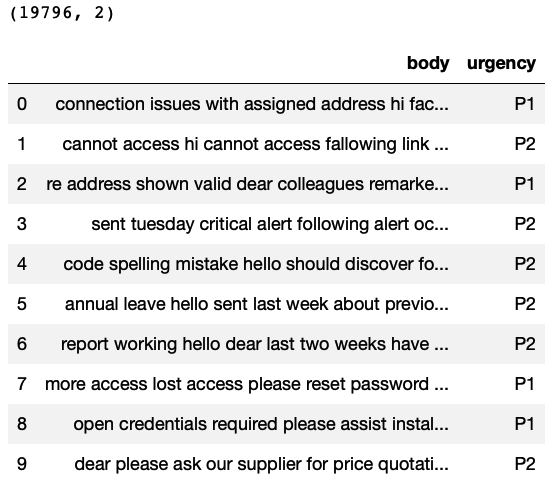
This data contains 19,796 rows and 2 columns. The column”body” represents the ticket description and the column “urgency” represents the Priority.
|
1 2 3 4 5 6 7 8 9 10 11 |
import pandas as pd import numpy as np # Reading the data TicketData=pd.read_csv('supportTicketData.csv') # Printing number of rows and columns print(TicketData.shape) # Printing sample rows TicketData.head(10) |
Visualising the distribution of the Target variable
Now we try to see if the Target variable has balanced distribution or not? Basically each priority type has enough number of rows to be learned.
If the data would have been imbalanced, for example very less number of rows for P1 category, then you need to balance the data using any of the popular techniques like over-sampling, under-sampling or SMOTE.
|
1 2 3 4 5 6 7 |
# Number of unique values for urgency column # You can see there are 3 ticket types print(TicketData.groupby('urgency').size()) # Plotting the bar chart %matplotlib inline TicketData.groupby('urgency').size().plot(kind='bar'); |

The above bar plot shows that there are enough rows for each ticket type. Hence, this is balanced data for classification.
TF-IDF Vectorization: converting text data to numeric
Now we will convert the text column “body” into TF-IDF matrix of numbers using TfidfVectorizer from sklearn library. This will get the text data into the numeric form, which will be learned by machine learning algorithms.
|
1 2 3 4 5 6 7 8 9 10 11 12 13 14 15 16 17 18 19 20 21 |
# TF-IDF vectorization of text from sklearn.feature_extraction.text import TfidfVectorizer from sklearn.feature_extraction.stop_words import ENGLISH_STOP_WORDS # Ticket Data corpus = TicketData['body'].values # Creating the vectorizer vectorizer = TfidfVectorizer(stop_words='english') # Converting the text to numeric data X = vectorizer.fit_transform(corpus) #print(vectorizer.get_feature_names()) # Preparing Data frame For machine learning # Priority column acts as a target variable and other columns as predictors DataForML=pd.DataFrame(X.toarray(), columns=vectorizer.get_feature_names()) DataForML['Priority']=TicketData['urgency'] print(DataForML.shape) DataForML.head() |

The above output is just a sample of the 19796 rows and 9100 columns!
Notice that the number of rows are same as the original data, but, the number of columns have exploded to 9100!!
This is because there were so many unique words in the support ticket texts even after removing the stop-words… 9099 unique words still remains, plus one Target variable “Priority”, hence, total 9100 columns.
The Curse of High Dimensionality
If we pass the above data to any machine learning algorithm, it will simply hang it! Especially the tree based algorithms. This is because of the sheer number of columns to process!
This problem is common in TF-IDF Vectorization because of the way it finds the representation for each sentence. Overall number of columns are bound to be very high because these are the unique words from all the text data!
This is exactly when we use Dimension Reduction! To represent the high number of columns with a lower number of columns.
Look at the below video to understand this concept in-depth!
Dimension Reduction
There are too many predictor columns(9099!), hence we use PCA to reduce the number of columns.
To select the best number of principal components, we need to run PCA once with the number of components equal to the number of columns, in this case 9099.
But, in the below snippet I am trying out 5000 maximum Principal Components. Why 5000? Because the total number of columns in original data is 9099 and that will take some time to process, hence I am just checking if the optimum number of components can be found below 5000 principal components or not? Luckily you see, the saturation was found near 2100 components.
Based on the cumulative variance explained chart, I will select the minimum number of principal components which can explain maximum amount of data variance. This is that point where the graph becomes horizontal.
Warning: Please run all the below codes on Google Colab or any other cloud platform. So that your laptop is not hanged due to the high amount of processing required!
|
1 2 3 4 5 6 7 8 9 10 11 12 13 14 15 16 17 18 19 20 21 22 23 24 25 26 27 28 29 30 31 32 |
''' #### Dimension Reduction #### ''' from sklearn.decomposition import PCA import matplotlib.pyplot as plt # Subsetting data for X and y TargetVariable=DataForML.columns[-1] Predictors=DataForML.columns[:-1] X=DataForML[Predictors].values y=DataForML[TargetVariable].values # Trying maximum 5000 components # You need to choose any number which is less than the total number of columns in the original data # I chose 5000 just to check if saturation happens before 5000 components or not. NumComponents=5000 pca = PCA(n_components=NumComponents) # fitting the data pca_fit=pca.fit(X) # calculating the principal components reduced_X = pca_fit.transform(X) #Cumulative Variance explained by each component var_explained_cumulative=np.cumsum(np.round(pca.explained_variance_ratio_, decimals=4)*100) print(var_explained_cumulative) # Look for the elbow in the plot plt.plot( range(1,len(var_explained_cumulative)+1), var_explained_cumulative ) plt.xlabel('Number of components') plt.ylabel('% Variance explained') |

Based on the above chart we can see that saturation is happening around 2100 principal components. They are explaining around 97% of the total data variance.
Hence choosing 2100 Principal components. With this, we were able to reduce the total number of columns significantly as compared to original 9099 predictor columns.
|
1 2 3 4 5 6 7 8 9 |
# Creating 2100 Principal components based on the above curve NumComponents=2100 pca = PCA(n_components=NumComponents) # fitting the data pca_fit=pca.fit(X) # calculating the principal components reduced_X = pca_fit.transform(X) |
Using Principal Components as predictors
Now combining the Target variable with the principal components and preparing the data for machine learning.
|
1 2 3 4 5 |
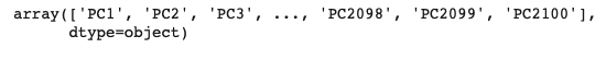
# Equating reduced_X to X to let the other code run without changing everything X=reduced_X # Generating Predictor names Predictors=pd.Series(['PC']*NumComponents).str.cat(pd.Series(range(1,NumComponents+1)).apply(str)).values Predictors |
Standardization/Normalization of the data
This is an optional step. It can speed up the processing of the model training.
|
1 2 3 4 5 6 7 8 9 10 11 12 13 14 15 16 17 18 19 20 21 22 23 |
from sklearn.preprocessing import StandardScaler, MinMaxScaler # Choose either standardization or Normalization # On this data Min Max Normalization is needed as we are fitting Naive Bayes # Choose between standardization and MinMAx normalization #PredictorScaler=StandardScaler() PredictorScaler=MinMaxScaler() # Storing the fit object for later reference PredictorScalerFit=PredictorScaler.fit(X) # Generating the standardized values of X X=PredictorScalerFit.transform(X) # Split the data into training and testing set from sklearn.model_selection import train_test_split X_train, X_test, y_train, y_test = train_test_split(X, y, test_size=0.3, random_state=428) # Sanity check for the sampled data print(X_train.shape) print(y_train.shape) print(X_test.shape) print(y_test.shape) |

Training ML classification models
Normally, while training classification models, we can use all of the famous classification algorithms like Random Forest, XGBoost, Adaboost, ANN etc.
But, this data is high dimensional even after dimension reduction! If you pass this data of 2100 columns to any of these algorithms then, it will take a while before it finishes training and if you are using your humble laptop CPU, it may even hang it!
So, while keeping the training speed in mind. I select below algorithms.
- Naive bayes
- Logistic Regression
- Decision Trees
Naive Bayes and Logistic Regression will run faster on such high dimensional data. I have kept Decision trees just for helping you to visualize how slow the training is for tree based models on such datasets.
Naive Bayes
This algorithm trains very fast! The accuracy may not be very high always but the speed is guaranteed! Hence you can even skip the dimension reduction step for Naive Bayes and get better accuracy by using the original data with 9099 columns.
Here the output is shown based on 2100 principal components, hence the lower accuracy. If you use the original data then this accuracy will go to 70%.
I have commented the cross validation section just to save computing time. You can uncomment and execute those commands as well.
|
1 2 3 4 5 6 7 8 9 10 11 12 13 14 15 16 17 18 19 20 21 22 23 24 25 26 27 28 29 30 31 32 33 34 35 36 37 38 39 40 |
# Naive Bays from sklearn.naive_bayes import GaussianNB, MultinomialNB # GaussianNB is preferred in Binomial Classification # MultinomialNB is preferred in multi-class classification clf = GaussianNB() #clf = MultinomialNB() # Printing all the parameters of Naive Bayes print(clf) # Generating the Naive Bayes model NB=clf.fit(X_train,y_train) # Generating predictions on testing data prediction=NB.predict(X_test) # Printing sample values of prediction in Testing data TestingData=pd.DataFrame(data=X_test, columns=Predictors) TestingData[TargetVariable]=y_test TestingData['Prediction']=prediction print(TestingData.head()) # Measuring accuracy on Testing Data from sklearn import metrics print(metrics.classification_report(y_test, prediction)) print(metrics.confusion_matrix(y_test, prediction)) # Printing the Overall Accuracy of the model F1_Score=metrics.f1_score(y_test, prediction, average='weighted') print('Accuracy of the model on Testing Sample Data:', round(F1_Score,2)) # Importing cross validation function from sklearn #from sklearn.model_selection import cross_val_score ## Running 10-Fold Cross validation on a given algorithm ## Passing full data X and y because the K-fold will split the data and automatically choose train/test #Accuracy_Values=cross_val_score(NB, X , y, cv=5, scoring='f1_weighted') #print('\nAccuracy values for 5-fold Cross Validation:\n',Accuracy_Values) #print('\nFinal Average Accuracy of the model:', round(Accuracy_Values.mean(),2)) |

Logistic Regression
This algorithm also trains very fast, but not as fast as Naive Bayes! However this slow speed comes with the nice tradeoff of accuracy! It produces more accurate results. In the below snippet you can see the accuracy as 73%
|
1 2 3 4 5 6 7 8 9 10 11 12 13 14 15 16 17 18 19 20 21 22 23 24 25 26 27 28 29 30 31 32 33 34 35 36 37 38 |
# Logistic Regression from sklearn.linear_model import LogisticRegression # choose parameter Penalty='l1' or C=1 # choose different values for solver 'newton-cg', 'lbfgs', 'liblinear', 'sag', 'saga' clf = LogisticRegression(C=5,penalty='l2', solver='newton-cg') # Printing all the parameters of logistic regression # print(clf) # Creating the model on Training Data LOG=clf.fit(X_train,y_train) # Generating predictions on testing data prediction=LOG.predict(X_test) # Printing sample values of prediction in Testing data TestingData=pd.DataFrame(data=X_test, columns=Predictors) TestingData[TargetVariable]=y_test TestingData['Prediction']=prediction print(TestingData.head()) # Measuring accuracy on Testing Data from sklearn import metrics print(metrics.classification_report(y_test, prediction)) print(metrics.confusion_matrix(prediction, y_test)) # Printing the Overall Accuracy of the model F1_Score=metrics.f1_score(y_test, prediction, average='weighted') print('Accuracy of the model on Testing Sample Data:', round(F1_Score,2)) # Importing cross validation function from sklearn #from sklearn.model_selection import cross_val_score # Running 10-Fold Cross validation on a given algorithm # Passing full data X and y because the K-fold will split the data and automatically choose train/test #Accuracy_Values=cross_val_score(LOG, X , y, cv=10, scoring='f1_weighted') #print('\nAccuracy values for 10-fold Cross Validation:\n',Accuracy_Values) #print('\nFinal Average Accuracy of the model:', round(Accuracy_Values.mean(),2)) |

Decision Trees
This algorithm will train painfully slow on such data! By looking at this you can imagine how slow a RandomForest or XGBoost will train! Hence, I have not included them in this case study.
|
1 2 3 4 5 6 7 8 9 10 11 12 13 14 15 16 17 18 19 20 21 22 23 24 25 26 27 28 29 30 31 32 33 34 |
# Decision Trees from sklearn import tree #choose from different tunable hyper parameters clf = tree.DecisionTreeClassifier(max_depth=5,criterion='gini') # Printing all the parameters of Decision Trees print(clf) # Creating the model on Training Data DTree=clf.fit(X_train,y_train) prediction=DTree.predict(X_test) # Measuring accuracy on Testing Data from sklearn import metrics print(metrics.classification_report(y_test, prediction)) print(metrics.confusion_matrix(y_test, prediction)) # Printing the Overall Accuracy of the model F1_Score=metrics.f1_score(y_test, prediction, average='weighted') print('Accuracy of the model on Testing Sample Data:', round(F1_Score,2)) # Plotting the feature importance for Top 10 most important columns %matplotlib inline feature_importances = pd.Series(DTree.feature_importances_, index=Predictors) feature_importances.nlargest(10).plot(kind='barh') # Importing cross validation function from sklearn from sklearn.model_selection import cross_val_score # Running 10-Fold Cross validation on a given algorithm # Passing full data X and y because the K-fold will split the data and automatically choose train/test #Accuracy_Values=cross_val_score(DTree, X , y, cv=10, scoring='f1_weighted') #print('\nAccuracy values for 10-fold Cross Validation:\n',Accuracy_Values) #print('\nFinal Average Accuracy of the model:', round(Accuracy_Values.mean(),2)) |

Training the best model on Full Data
Based on the above outputs, we select Logistic Regression as the final model.
|
1 2 3 4 5 6 7 |
# Generating the Logistic Regression model on full data # This is the best performing model from sklearn.linear_model import LogisticRegression # choose parameter Penalty='l1' or C=1 # choose different values for solver 'newton-cg', 'lbfgs', 'liblinear', 'sag', 'saga' clf = LogisticRegression(C=5,penalty='l2', solver='newton-cg') FinalModel=clf.fit(X,y) |
Making predictions for New Cases
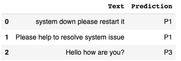
This final model is deployed in production to classify the new incoming tickets. To do this, we write a function which can generate predictions either one at a time OR for multiple cases input as a data frame.
|
1 2 3 4 5 6 7 8 9 10 11 12 13 14 15 16 17 18 19 20 |
# Defining a function which converts words into numeric vectors for prediction def FunctionPredictUrgency(inpText): # Using the same vectorizer converting the text to numeric vector X=vectorizer.transform(inpText) #print(X.toarray()) # calculating the principal components reduced_X = pca_fit.transform(X.toarray()) # If standardization/normalization was done on training # then the above X must also be converted to same platform # Generating the normalized values of X X=PredictorScalerFit.transform(reduced_X) # Generating the prediction using Naive Bayes model and returning Prediction=FinalModel.predict(X) Result=pd.DataFrame(data=inpText, columns=['Text']) Result['Prediction']=Prediction return(Result) |
|
1 2 3 4 |
# Calling the function NewTicket=["system down please restart it", "Please help to resolve system issue","Hello how are you?"] PredictionResults=FunctionPredictUrgency(inpText=NewTicket) PredictionResults |
Saving the output as a file
You can write the PredictionResults dataframe as a csv or excel file. And then from there it can be loaded into the database.
|
1 2 |
# Saving the results as a csv file PredictionResults.to_csv('PredictionResults.csv',index=False) |
Conclusion
I hope this post was helpful for you to get a practical flow of Text Vectorization using TF-IDF and you will be able to apply this in your projects. Consider sharing this post with your friends to spread the knowledge and help me grow as well!

Hi Farukh, I hope this message finds u well. I have been reading your content for about a week and I am absolutely loving it. I have watched many videos and read so many articles about ML and Data science , but I didn’t like any of them as they lack anyone of the aspect of the total workflow. As I am New grad, I was searching for resources that can get me understand what ML is like in industries. Your content has made ML easy to understand and interesting . I hope You are going to give like this content much more in the future. I am very eager to learn from you knowledge. Thank you so much for the GOD level content.
I hope we can connect and share our thoughts.
You are a saviour.
Good day and Thank you.
Hi Vinsy,
I am glad that the blog helped you!
Thank you for the kind words!
This motivates me to work more!
Regards,
Farukh Hashmi
Nicely explained. Thank you