In the previous post, I talked about the popular supervised machine learning algorithms. In this post, I will discuss some of the important Unsupervised machine learning algorithms which are asked in the data science interviews.
I will also show you, how to run these algorithms in R/Python.
Table of contents
- Overview
- K-Means
- Hierarchical Clustering
- DBSCAN
- OPTICS
- Factor Analysis
- Factor Analysis Vs PCA
- PCA
- ICA
- T-SNE
- UMAP
- Association Rule Mining
- Apriori
- Eclat
- FP-Growth
Overview
Unsupervised means without any intervention. These algorithms do not need supervision to learn about the data. It means you don’t have to explicitly ‘train’ them by telling this is the input(X) and that is the output(y).
Unsupervised machine learning is about finding the patterns in data by just passing full data to the algorithm.
Unsupervised machine learning algorithms do not need supervision to learn about the data. It means you don’t have to explicitly ‘train’ them by telling this is the input(X) and that is the output(y).
Clustering, Dimension Reduction, and Association are the three major types of tasks that are performed by Unsupervised Machine Learning algorithms.

Clustering: Finding groups of data. Basically, put similar ROWS in data under one group. For example,
- Finding the types of customers using shopping behavior data
- Finding the types of users in telecom, based on their usage data.
- How many groups are present in a given unknown data.
Important algorithms used for clustering are K-Means, Hierarchical clustering, DBSCAN, and OPTICS.
Dimension Reduction: Finding and combining similar columns in data. Basically reducing the number of columns(Dimension) to a lower number of columns.
Important algorithms used for Dimension Reduction are Factor Analysis, PCA, ICA, T-SNA, and UMAP.
Association: Finding out the patterns in the customer purchase behavior and generating the purchase recommendations. Basically, if a user purchases item-A, then which item they will likely purchase along with it.
Important algorithms used for Association are Apriori, Eclat, and FP-Growth.
Let’s discuss these algorithms one by one!
Q How does the K-Means clustering algorithm work?

K-Means Algorithm is a simple yet powerful Unsupervised machine learning algorithm.
It is used to find groups/clusters of similar rows in data.
The working of K-Means is simple. Pass the data, tell how many clusters you want and K-Means will assign a group to every row in data.
Please look at the K-Means algorithm steps below
- If the value of K=2, then we need to find 2 groups in data
- Assign group-1 or group-2 label to each observation in the data randomly
- Find the “center” of all group-1 points and all group-2 points. These centers are known as “centroids”
- Find the distances of each point from both the “centroids”
- Assign each point to the nearest centroid. Hence, the corresponding group.
- Repeat steps 3-5 till there are no further changes in the positions of the centroids OR the maximum number of iterations are completed.
- In the end, each observation in data is assigned to one of the groups.

data –> K-Means(find 2 groups) –> Found 2 groups
On the same data, if you ask K-Means to find 3 groups, the algorithm will find you 3 groups as well!
data –> K-Means(find 3 groups) –> Found 3 groups
How do we find the optimal number of groups in data?
By running the process iteratively for K=1, 2, 3, 4…10 and noting down the “withinness” i.e. the similarity between all points within a group. This is measured as the sum of the distances of each point from the centroid.
If all the points are close to the centroid, that means the group is homogeneous. i.e. all observations are very similar.
Ideally, withinness should be Zero, but, in practice, we try to keep it as low as possible, since you never get Zero.
“Euclidean” distance is popular for withinness calculation.
Q. How to create K-Means in R?
|
1 2 3 4 5 6 7 8 9 10 11 12 13 14 15 16 17 18 19 20 21 22 23 24 25 26 27 28 29 30 31 32 33 34 35 36 37 38 39 40 41 42 43 44 45 46 |
# Sample code to create K-Means in R # Choose the data on which clustering has to be done # Always remove the target variable before passing the data for clustering # Using the famous IRIS data set and removing the target variable "Species" ClusterData=iris[, -5] head(ClusterData) # Create a data frame to store results IterationData=data.frame( numberOfClusters=numeric(0), Within_SS=numeric(0)) # Trying to find out best number of clusters present in the given data # Running K-Means 10 times and creating different number of clusters each time for (i in c(1:10)){ KmeansCluster=kmeans(ClusterData,i) IterationData=rbind(IterationData,data.frame( numberOfClusters=i, Within_SS=round(sum(KmeansCluster$withinss), 2)) ) } # Stopping R to abbreviate numbers to scientific notation options(scipen=100000) print('#### clustering iteration results ####') IterationData # By looking at the curve we can see 3 clusters are optimal # Due to the elbow found at K=3 plot(IterationData$numberOfClusters,IterationData$Within_SS) lines(IterationData$numberOfClusters,IterationData$Within_SS) ######################################################################## # Creating final number of clusters based on above curve OptimalClusters=kmeans(ClusterData,3) OptimalClusters ######################################################################## # Assigning cluster id for each row ClusterData$ClusterID=OptimalClusters$cluster head(ClusterData) ######################################################################## # Visualizing the clusters using first and third columns # Choose those two columns which has highest range # pch means plotting character # cex means magnification factor plot(ClusterData[,1], ClusterData[,3], col=ClusterData$ClusterID, pch='*', cex=2) |
Q. How to create K-Means in Python?
|
1 2 3 4 5 6 7 8 9 10 11 12 13 14 15 16 17 18 19 20 21 22 23 24 25 26 27 28 29 30 31 32 33 34 35 36 37 38 39 40 41 42 43 44 45 46 47 48 49 50 51 52 53 |
# Sample code to create K-Means in Python # Creating the sample data for clustering from sklearn.datasets import make_blobs import matplotlib.pyplot as plt import numpy as np import pandas as pd # create sample data for clustering SampleData =make_blobs(n_samples=100,n_features=2,centers=2,cluster_std=1.5,random_state=40) #create np array for data points X = SampleData[0] y=SampleData[1] # Creating a Data Frame to represent the data with labels ClusterData=pd.DataFrame(list(zip(X[:,0],X[:,1],y)), columns=['X1','X2','ClusterID']) print(ClusterData.head()) # create scatter plot to visualize the data %matplotlib inline plt.scatter(ClusterData['X1'], ClusterData['X2'], c=ClusterData['ClusterID']) ################################################################################## from sklearn.cluster import KMeans import matplotlib.pyplot as plt # Creating Empty List to store Inertia value Intertia = [] # Running K-Means 10 times to find the optimal number of clusters for i in range(1, 11): km = KMeans(n_clusters=i, n_init=10, max_iter=300, random_state=0) km.fit(X) Intertia.append(km.inertia_) # Plotting the curve to find the optimal number of clusters # That point where the line starts to become horizontal is the ideal value plt.plot(range(1, 11), Intertia, marker='o') plt.xlabel('Number of clusters') plt.ylabel('Inertia') plt.tight_layout() plt.show() # Creating 2 Clusters Based on the above graph km = KMeans(n_clusters=2,n_init=10, max_iter=300, random_state=0) km.fit(X) ClusterData['PredictedClusterID']=km.predict(X) print(ClusterData.head()) # Plotting the predicted clusters plt.scatter(ClusterData['X1'], ClusterData['X2'], c=ClusterData['PredictedClusterID']) |
Q How does the Hierarchical clustering algorithm work?

Hierarchical clustering is another algorithm that helps to group similar rows together.
Hierarchical clustering algorithm has two major types listed below
- Agglomerative (Bottom-Up Approach)
- Divisive (Top-Down Approach)
Agglomerative Clustering is a Bottom-Up approach, it works with the below steps.
- Assume every row is one cluster in itself, so if your data has 100 rows then start at the bottom with 100 clusters
- Compute the distance matrix of every cluster from every other cluster using a distance measure, e.g Euclidean/Manhattan. For text data/other non-numeric data we use Hamming or Levenshtein distance.
- Use the above distance matrix to calculate the distances between the clusters. The cluster distances can be of 3 types:
- Single Linkage (The shortest distance between two clusters)
- Complete Linkage (The largest distance between two clusters)
- Average Linkage (The average distance between two clusters)
- Find which clusters are closest to each other
- Combine all those clusters that are closest to each other.
- keep repeating steps 2-5 until there is only 1 cluster left.

The above iterative process creates a chart known as the Dendrogram.
This diagram helps us to select the optimal number of clusters in the data.
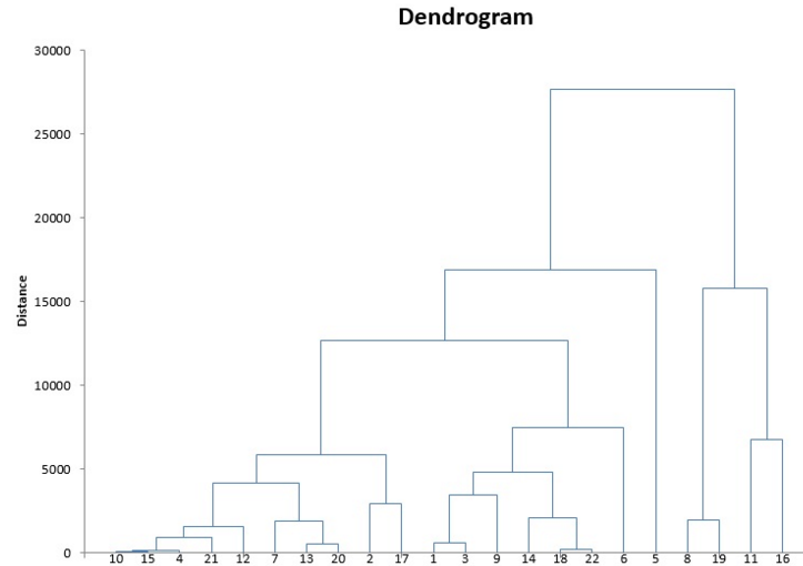
If I “cut” the dendrogram at Distance=20,000, then I will get 2 clusters
If I “cut” the dendrogram at Distance=15,000, then I will get 4 clusters.
If I “cut” the dendrogram at Distance=10,000, then I will get 5 clusters.
So which one is the best? Where exactly to cut the Dendrogram?
We cut the dendrogram at the point where the horizontal line covers the maximum distance between 2 vertical lines.
Hence, we make sure the clusters are as far as possible. In the below scenario, we will cut the dendrogram at Distance=10,000. It will fetch us 5 clusters from the data.

Divisive Clustering (Top-Down approach) is exactly the opposite of Agglomerative. Start from the top with all rows in one cluster and keep dividing the clusters unless every row is one cluster in itself.
Q. How to create Hierarchical clustering in R?
|
1 2 3 4 5 6 7 8 9 10 11 12 13 14 15 16 17 18 19 20 21 22 23 24 25 26 27 28 29 30 31 32 33 34 |
# Sample code to create Hierarchical Clustering in R # Choose the data on which clustering has to be done # Always remove the target variable before passing the data for clustering # Using the famous IRIS data set and removing the target variable "Species" ClusterData=iris[, -5] head(ClusterData) # Computing the distance matrix DistanceMatrix=dist(ClusterData) # Creating the Hirarchical clusters Hcluster=hclust(DistanceMatrix) # Plotting the dendrogram to check how many clusters to select plot(Hcluster) # Selecting the apt number of clusters by inspecting the dendrogram # Cutting the dendrogram to get 3 clusters using parameter k ClusterID=cutree(Hcluster, k=3) # Visualizing the dendrogram cut # Choosing height h=3.5 will cut the dendrogram for 3 clusters plot(Hcluster) abline(h = 3.5, col = "red") # Assigning cluster id for each row ClusterData$ClusterID=ClusterID head(ClusterData) # Visualizing the clusters using first and third columns # Choose those two columns which has highest range # pch means plotting character # cex means magnification factor plot(ClusterData[,1], ClusterData[,3], col=ClusterData$ClusterID, pch='*', cex=2) |
Q. How to create Hierarchical clustering in Python?
|
1 2 3 4 5 6 7 8 9 10 11 12 13 14 15 16 17 18 19 20 21 22 23 24 25 26 27 28 29 30 31 32 33 34 35 36 37 38 39 40 41 42 |
# Sample code to create Hierarchical Clustering in Python # Creating the sample data for clustering from sklearn.datasets import make_blobs import matplotlib.pyplot as plt import numpy as np import pandas as pd # create sample data for clustering SampleData = make_blobs(n_samples=100, n_features=2, centers=2, cluster_std=1.5,random_state=40) #create np array for data points X = SampleData[0] y=SampleData[1] # Creating a Data Frame to represent the data with labels ClusterData=pd.DataFrame(list(zip(X[:,0],X[:,1],y)), columns=['X1','X2','ClusterID']) print(ClusterData.head()) # create scatter plot to visualize the data %matplotlib inline plt.scatter(ClusterData['X1'], ClusterData['X2'], c=ClusterData['ClusterID']) ################################################################################## # create dendrogram to find best number of clusters import scipy.cluster.hierarchy as sch dendrogram = sch.dendrogram(sch.linkage(X, method='ward')) # Creating 2 Clusters Based on the above dendogram visually Bottom-Up hierarchical clustering from sklearn.cluster import AgglomerativeClustering hc = AgglomerativeClustering(n_clusters=2, affinity = 'euclidean', linkage = 'ward') # Generating cluster id for each row using agglomerative algorithm ClusterData['PredictedClusterID']=hc.fit_predict(X) print(ClusterData.head()) #Plotting the predicted clusters plt.scatter(ClusterData['X1'], ClusterData['X2'], c=ClusterData['PredictedClusterID']) # Use of Linkage # "ward" minimizes the variance of the clusters being merged. #"average" uses the average of the distances of each observation of the two sets. # "complete" or maximum linkage uses the maximum distances between all observations of the two sets. |
Q How does the DBSCAN clustering algorithm work?

DBSCAN stands for Density Based Spatial Clustering of Applications with Noise.
Do not get intimidated by this algorithm’s name, the more it sounds complex the simpler it is actually! 🙂
Lets quickly understand the relevant terminologies for DBSCAN.
- ε, epsilon (eps): is known as the maximum allowed distance from one point to the other point, for both of them to be considered in one group/cluster
- MinPts: is the minimum number of points which should be present close to each other at a distance of epsilon (ε) so that they all can be form a group/cluster
- Core Point: That point which has at least MinPts number of points near to it, within the distance of ε(eps)
- Border Point/Non-Core Point: That point in data which has less than the minimum number of points(MinPts) within its reach (a distance of eps)
- Noise: That point which has no point near to it within a distance of eps
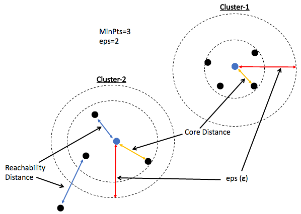
In the below diagram, the minimum distance required (eps) is 2 units and the minimum number of points which must be near to the core point is 3.

You can observe in the above diagram:
- The core point has 4 points within its circle of 2 units.
- The Border point has only one point(Blue Point) near to it and hence it is not a core point.
- The Noise (Red Point) has no points within its circle hence it is labeled as noise. Because it does not belong to any group/cluster
The DBSCAN algorithm is very simple. Look at its working steps below:
- Start with one point randomly, find out if it is a core point by checking the minimum number of points near to it by a distance of eps
- If it is a core point, make it a cluster and move to the next unvisited point to repeat step-1
- If the number of points within eps distance is fewer than MinPts then mark it as non-core point
- If the number of points within eps distance is Zero, then mark that point as Noise.
- Combine all those clusters together whose points are within eps distance. Also known as density connection or connected components. This starts a chain reaction. If cluster-1 and cluster-2 are connected and cluster-2 and cluster-3 are connected then cluster-1 and cluster-3 are also connected. Hence all these are combined to make one single cluster.

Q. How to create DBSCAN clustering in R?
|
1 2 3 4 5 6 7 8 9 10 11 12 13 14 15 16 17 18 19 20 21 22 23 24 25 |
# Sample code to create DBSCAN Clustering in R # Choose the data on which clustering has to be done # Always remove the target variable before passing the data for clustering # Using the famous IRIS data set and removing the target variable "Species" ClusterData=iris[, -5] head(ClusterData) # Creating Clusters using DBSCAN algorithm library(dbscan) DBSCANclusters=dbscan(ClusterData, eps = 0.5, minPts = 5) print(DBSCANclusters) # Visualizing the clusters created and Noize points hullplot(ClusterData, DBSCANclusters) # Assigning cluster id for each row # Adding 1 to clusterID to make the 0 values visible in plot ClusterData$ClusterID=DBSCANclusters$cluster+1 head(ClusterData) # Visualizing the clusters using first and third columns # Choose those two columns which has highest range # pch means plotting character # cex means magnification factor plot(ClusterData[,1], ClusterData[,3], col=ClusterData$ClusterID, pch='*', cex=2) |
Q. How to create DBSCAN clustering in Python?
|
1 2 3 4 5 6 7 8 9 10 11 12 13 14 15 16 17 18 19 20 21 22 23 24 25 26 27 28 29 30 31 32 33 34 35 36 37 38 39 40 41 |
# Sample code to create DBSCAN Clustering in Python # Creating the sample data for clustering from sklearn.datasets import make_blobs import matplotlib.pyplot as plt import numpy as np import pandas as pd # create sample data for clustering SampleData = make_blobs(n_samples=100, n_features=2, centers=2, cluster_std=1.5, random_state=40) #create np array for data points X = SampleData[0] y=SampleData[1] # Creating a Data Frame to represent the data with labels ClusterData=pd.DataFrame(list(zip(X[:,0],X[:,1],y)), columns=['X1','X2','ClusterID']) print(ClusterData.head()) # create scatter plot to visualize the data %matplotlib inline plt.scatter(ClusterData['X1'], ClusterData['X2'], c=ClusterData['ClusterID']) ################################################################################## from sklearn.cluster import DBSCAN db = DBSCAN(eps=1, min_samples=5) # Generating cluster id for each row using DBSCAN algorithm # -1 indicates the point is a noize, and does not belong to any cluster ClusterData['PredictedClusterID']=db.fit_predict(X) print(ClusterData.head()) # Plotting the predicted clusters plt.scatter(ClusterData['X1'], ClusterData['X2'], c=ClusterData['PredictedClusterID']) # eps : float, optional # The maximum distance between two samples for them to be considered # as in the same neighborhood. # min_samples : int, optional # The number of samples (or total weight) in a neighborhood for a point # to be considered as a core point. This includes the point itself. |
Q How does the OPTICS clustering algorithm work?

OPTICS stands for Ordering Points To Identify Clustering Structure.
Once again another fancy name but a very simple algorithm!
This algorithm can be seen as a generalization of DBSCAN. A major issue with DBSCAN is that it fails to find clusters of varying density due to fixed eps.
This is solved in OPTICS by using an approach of finding reachability of each point from the core points and then deciding the clusters based on reachability plot.
Lets quickly understand the relevant terminologies for OPTICS.
- ε, epsilon (eps): is known as the Maximum allowed distance from one point to the other point for both of them to be considered in one group/cluster
- MinPts: is the minimum number of points which should be present close to each other at a distance of epsilon (ε) so that they all can be form a group/cluster
- Core Point: That point which has at least MinPts number of points near to it, within the distance of ε(eps)
- Border Point/Non-Core Point: That point in data which has less than the minimum number of points(MinPts) within its reach (a distance of eps)
- Noise: That point which has no point near to it within a distance of eps
In addition to the above, there are two additional terminologies which are used in OPTICS:
- Core Distance: The minimum distance required by a point to become a core point. It means it is possible to find the MinPts number of points within this distance. Core distance can be less than the pre-decided value of ε, epsilon (eps), which is the maximum allowed distance to find MinPts.
- Reachability distance: This is the distance to reach a point from the cluster. Now if the point lies within the Core Distance, then Reachability Distance=Core Distance. And, if the point lies outside the Core Distance, then Reachability Distance is the minimum distance from the extreme point of the cluster.
The OPTICS algorithm works with below steps:
- For the given values of MinPts and eps(ε). Find out if a point is close to MinPts number of points within a distance less than or equal to eps. Tag it as a Core Point. Update the reachability distance = core distance for all the points within the cluster.
- If it is not a core point then find out its density connected distance from the nearest cluster. Update the reachability distance.
- Arrange the data in increasing order of reachability distance for each cluster. The smallest distances come first and represent the dense sections of data and the largest distances come next representing the noise section. This is a special type of dendrogram
- Find out the places where a sharp decline is happening in the reachability distance plot.
- “Cut” the plot in the y-axis by a suitable distance to get the clusters.
Basically those points which are close to each other and form a dense cluster will have small reachability distance and those points which are far away from all the clusters are Noize points, they don’t belong to any of the clusters.
In the below plot, you can see the reachability distances of all the points ordered. A sudden decline marks the starting of a new cluster.
Clusters are created by inspecting this graph and choosing an appropriate reachability distance threshold to define the clusters. In the below plot, I have used Reachability Distance=0.5 as the threshold. This can also be done automatically by providing a measure of sharp decline known as “Xi“. Its value varies between 0 to 1. Higher the value, sharper the decline in the plot.


Q. How to create OPTICS clustering in R?
|
1 2 3 4 5 6 7 8 9 10 11 12 13 14 15 16 17 18 19 20 21 22 23 24 25 26 27 28 29 30 31 32 33 34 |
# Sample code to create OPTICS Clustering in R # Choose the data on which clustering has to be done # Always remove the target variable before passing the data for clustering # Using the famous IRIS data set and removing the target variable "Species" ClusterData=iris[, -5] head(ClusterData) # Creating Clusters using OPTICS algorithm library(dbscan) OPTICSclusters=optics(ClusterData, eps = 2, minPts = 5) OPTICSclusters # Extract the Rechability Distances by cutting the reachability plot at eps_cl RechabilityDistances=extractDBSCAN(OPTICSclusters, eps_cl = 0.5) # Plotting the reachability distances to see cluster formation # Black lines are noise plot(RechabilityDistances) # Visualizing the clusters created and Noize points hullplot(ClusterData, RechabilityDistances) # extract Clusters of varying density using the Xi method XiClusters=extractXi(OPTICSclusters, xi = 0.05) # Assigning cluster id for each row ClusterData$ClusterID=XiClusters$cluster head(ClusterData) # Visualizing the clusters using first and third columns # Choose those two columns which has highest range # pch means plotting character # cex means magnification factor plot(ClusterData[,1], ClusterData[,3], col=ClusterData$ClusterID, pch='*', cex=2) |
Q. How to create OPTICS clustering in Python?
|
1 2 3 4 5 6 7 8 9 10 11 12 13 14 15 16 17 18 19 20 21 22 23 24 25 26 27 28 29 30 31 32 33 34 |
# Sample code to create OPTICS Clustering in Python # Creating the sample data for clustering from sklearn.datasets import make_blobs import matplotlib.pyplot as plt import numpy as np import pandas as pd # create sample data for clustering SampleData = make_blobs(n_samples=100, n_features=2, centers=2, cluster_std=1.5, random_state=40) #create np array for data points X = SampleData[0] y=SampleData[1] # Creating a Data Frame to represent the data with labels ClusterData=pd.DataFrame(list(zip(X[:,0],X[:,1],y)), columns=['X1','X2','ClusterID']) print(ClusterData.head()) # create scatter plot to visualize the data %matplotlib inline plt.scatter(ClusterData['X1'], ClusterData['X2'], c=ClusterData['ClusterID']) ################################################################################## # This function is not present in python version 3.6 # Other option is pyclustering.cluster.optics but its not neat from sklearn.cluster import OPTICS op = OPTICS(min_samples=50, xi=.05, min_cluster_size=.05) # Generating cluster id for each row using DBSCAN algorithm ClusterData['PredictedClusterID']=op.fit_predict(X) print(ClusterData.head()) # Plotting the predicted clusters plt.scatter(ClusterData['X1'], ClusterData['X2'], c=ClusterData['PredictedClusterID']) |
Q How does the Factor Analysis algorithm work?

Factor analysis is a dimension reduction technique. The goal is to find out latent factors or hidden groups that are responsible for the observed data in the variables.
For example, if an employee is unhappy in an organization, there could be many reasons for it, but, if looked carefully, these reasons can be grouped together within some smaller set of MAJOR reasons! Factor analysis helps us find these major groups of variables in the data which are also known as Factors.
Factor analysis helps us find hidden groups(Factors) of variables in the data automatically
Look at the diagram below, it represents data from an employee survey. It shows the average ratings for each department, like how employees feel about the way their employer handles the complaints, how they feel about the privileges provided, how they feel about the learnings on the job and how they feel about their salary raises and career advancement, etc.

You can see that some of these responses represent a common subject or the Major reasons for the way they responded, e.g. If they are satisfied with their organization’s work culture, then scores will be high for overall rating, complaints, and privileges. If they feel they are learning on the job then scores will be high for learning opportunities, similarly for Promotions.
So there are 3 major reasons Work culture, Learning Opportunities, and Promotions, which actually DRIVES the ratings of smaller reasons like rating, complaints, etc.
Statistically, you can imagine the equations of the above diagram as below:
rating= β1*(Work Culture) + C1
complaints=β2*(Work Culture) + C2
privileges=β3*(Work Culture) + C3
Learning= β4*(Learning Opportunities) + C4
raises= β5*(Promotions) + C5
Factor Analysis helps to find these coefficients β1, β2, β3… and C1, C2, C3… etc.
These coefficients determine that what is the weightage of rating/complaints/privileges in Work Culture Factor, what is the weightage of raises/critical/advance in Promotions Factor etc.
These weightages are also known as Factor Loadings. Basically, what part of a given variable contributes to the group/Factor it belongs to.
Factor Loadings are the coefficient values for each variable, which represents its weightage in the Factor it belongs to.
Factor Analysis Vs PCA
Factor Analysis is often confused with Principal Component Analysis PCA!
Both are dimension reduction techniques, but, the main difference between Factor Analysis and PCA is the way they try to reduce the dimensions.
Factor Analysis tries to find the hidden groups of variables, which is like a common driving factor for the type of values in all those variables, e.g. customer survey, if you are unhappy with the taste of the coffee then all those questions about coffee taste in the survey will have low scores! Hence Bad Taste will be a Factor and questions like Coffee sweetness rating, Coffee bitterness rating, Coffee Freshness rating will represent the individual variables that will have low ratings.
Factor Analysis will form equations like below:
Coffee sweetness rating = β1 * (Bad Taste) +C1
Coffee bitterness rating = β2 * (Bad Taste) +C2
Coffee Freshness rating = β3 * (Bad Taste) +C3
PCA tries to find fewer new variables called Principal Components which are linear combinations of the variables in the data, hence these fewer variables “represent” all the variables, while reducing the dimensions. Here the goal is to create a new dataset that has the same number of rows but, lesser number of columns(Principal Components) which explains the variance of all the original variables in the data.
PCA will form equations like below:
PC1=α1 * ( Coffee sweetness rating) + α2(Coffee bitterness rating) + α3(Coffee Freshness rating)
PC2=β1 * ( Coffee sweetness rating) + β2(Coffee bitterness rating) + β3(Coffee Freshness rating)
Q. How to do Factor Analysis in R?
|
1 2 3 4 5 6 7 8 9 10 11 12 13 14 15 16 17 18 19 20 21 22 |
# Sample code to do Factor Analysis in R # Using employee attitude survey data FactorData=attitude # Generating correlation matrix corrMatrix=cor(FactorData) # using the library psych for Factor Analysis library(psych) # Finding out how many Factors are actually present in the data using scree plot # fm = Factor Exatraction Method used, here we used Minimum Residual (OLS) # fa = show Factor Analysis results, fa="pc" shows results for Principal Components parallel=fa.parallel(corrMatrix, fm = 'minres', fa = 'fa') # From the above graph it is evident that there are 4 Factors in data # Creating 4 Factors Factors=fa(r = corrMatrix, nfactors = 4) Factors # Choosing the threshold of 0.3 for minimum loading print(Factors$loadings,cutoff = 0.3) |
Q. How to do Factor Analysis in Python?
|
1 2 3 4 5 6 7 8 9 10 11 12 13 14 15 16 17 18 19 20 21 22 23 24 25 26 27 28 29 30 31 32 33 34 35 36 37 38 39 40 41 42 43 44 |
# Sample code to do Factor Analysis in Python # Creating the employee attitude survey data for Factor Analysis rating=[43,63,71,61,81,43,58,71,72,67,64,67,69,68,77,81,74,65,65,50,50,64,53,40,63,66,78,48,85,82] complaints=[51,64,70,63,78,55,67,75,82,61,53,60,62,83,77,90,85,60,70,58,40,61,66,37,54,77,75,57,85,82] privileges=[30,51,68,45,56,49,42,50,72,45,53,47,57,83,54,50,64,65,46,68,33,52,52,42,42,66,58,44,71,39] learning=[39,54,69,47,66,44,56,55,67,47,58,39,42,45,72,72,69,75,57,54,34,62,50,58,48,63,74,45,71,59] raises=[61,63,76,54,71,54,66,70,71,62,58,59,55,59,79,60,79,55,75,64,43,66,63,50,66,88,80,51,77,64] critical=[92,73,86,84,83,49,68,66,83,80,67,74,63,77,77,54,79,80,85,78,64,80,80,57,75,76,78,83,74,78] advance=[45,47,48,35,47,34,35,41,31,41,34,41,25,35,46,36,63,60,46,52,33,41,37,49,33,72,49,38,55,39] #Joining all the vectors together to form input matrix X SurveyData=list(zip(rating,complaints,privileges,learning,raises,critical,advance)) import pandas as pd InpData=pd.DataFrame(data=SurveyData, columns=["rating","complaints","privileges","learning","raises","critical","advance"]) print(InpData.head(10)) #Creating input data numpy array X=InpData.values ###################################################################### # Exploratory Factor Analysis To find how many factors are present in the data # Finding how many factors are present in the data # Installing the required library #!pip install factor_analyzer from factor_analyzer import FactorAnalyzer fa = FactorAnalyzer() Factors=fa.fit(X) # Plotting the scree-plot EigenValues=Factors.get_eigenvalues()[0] import matplotlib.pyplot as plt %matplotlib inline plt.plot(EigenValues) # Creating 4 Factors based on the screeplot from sklearn.decomposition import FactorAnalysis FA=FactorAnalysis(n_components=4, random_state=0) Factors=FA.fit(X) # Printing Factor Loadings print(pd.DataFrame(FA.components_, columns=InpData.columns, index=['PC1','PC2','PC3','PC4'])) |
Q How does the PCA algorithm work?

PCA stands for Principal Components Analysis.
It is one of the most popular algorithms which is used for dimension reduction (Reducing the number of columns/variables in data).

PCA represents the whole data with the help of fewer variables called principal components. These fewer number of new columns account for all the variance in the original data!
PCA works with below steps
- Find linear combinations of variables in data like
- PC1=α1 * (rating) + α2(complaints) + α3(privileges). . .
- PC1=α1 * (rating) + α2(complaints) + α3(privileges). . .
- While satisfying the independence criteria of all principal components. If you pick any two principal components and find correlation between them, it should be Zero.
- The first principal component explains the maximum amount of variance in data, the second principal component explains slightly less amount of variance, so on and so forth…
Q. How to run PCA in R?
|
1 2 3 4 5 6 7 8 9 10 11 12 13 14 15 16 17 18 19 20 21 22 23 24 25 26 27 28 29 30 31 32 33 |
# Sample code to do PCA in R DataForPCA=attitude head(DataForPCA) # Creating unsupervised PCA model on Predictors PrincipalComponents=prcomp(DataForPCA,scale=T) # Taking out the summary of PCA PCASummary=data.frame(summary(PrincipalComponents)$importance) PCASummary # Column Names of PCASummary data.frame is Principal component names PrincipalComponents=1:ncol(PCASummary) # Third row of the data frame are cumulative variances IndividualVarianceExplained=PCASummary[2,] * 100 # Plotting the variances explained by each Principal Components plot(PrincipalComponents,IndividualVarianceExplained, main='Individual Variances') lines(PrincipalComponents,IndividualVarianceExplained) # Choosing Principal components based on above scree plot # Individual plot suggests to choose 5 Principal Components # This means we can represent all the data using only 5 variables # Generating principal components values PrincipalComponentValues=predict(PredictorPCA, PredictorVariablesDummies) head(PrincipalComponentValues) # Choosing Best number of Principal Components BestPrincipalComponents=PrincipalComponentValues[,c(1:5)] head(BestPrincipalComponents) |
Q. How to run PCA in Python?
|
1 2 3 4 5 6 7 8 9 10 11 12 13 14 15 16 17 18 19 20 21 22 23 24 25 26 27 28 29 30 31 32 33 34 35 36 37 38 39 40 41 42 43 44 45 46 47 48 |
# Sample code to do PCA in Python # Creating the employee attitude survey data for PCA rating=[43,63,71,61,81,43,58,71,72,67,64,67,69,68,77,81,74,65,65,50,50,64,53,40,63,66,78,48,85,82] complaints=[51,64,70,63,78,55,67,75,82,61,53,60,62,83,77,90,85,60,70,58,40,61,66,37,54,77,75,57,85,82] privileges=[30,51,68,45,56,49,42,50,72,45,53,47,57,83,54,50,64,65,46,68,33,52,52,42,42,66,58,44,71,39] learning=[39,54,69,47,66,44,56,55,67,47,58,39,42,45,72,72,69,75,57,54,34,62,50,58,48,63,74,45,71,59] raises=[61,63,76,54,71,54,66,70,71,62,58,59,55,59,79,60,79,55,75,64,43,66,63,50,66,88,80,51,77,64] critical=[92,73,86,84,83,49,68,66,83,80,67,74,63,77,77,54,79,80,85,78,64,80,80,57,75,76,78,83,74,78] advance=[45,47,48,35,47,34,35,41,31,41,34,41,25,35,46,36,63,60,46,52,33,41,37,49,33,72,49,38,55,39] #Joining all the vectors together to form input matrix X SurveyData=list(zip(rating,complaints,privileges,learning,raises,critical,advance)) import pandas as pd InpData=pd.DataFrame(data=SurveyData, columns=["rating","complaints","privileges","learning","raises","critical","advance"]) print(InpData.head(10)) #Creating input data numpy array X=InpData.values ###################################################################### # Creating maximum number of principal components from sklearn.decomposition import PCA pca = PCA(n_components=X.shape[1]) PrincipalComponents=pca.fit(X) # Finding the variance explained by each component import numpy as np var_explained= PrincipalComponents.explained_variance_ratio_ var_explained_cumulative=np.cumsum(np.round(var_explained, decimals=4)*100) # plotting the variance explained to find optimal number of components plt.plot(np.array(range(1,8)),var_explained_cumulative) # By Looking at below graph we can see that 5 components are explaining maximum Variance # in the dataset the elbow/saturation occurs at 5th principal component # choosing 5 principal components based on above graph pca = PCA(n_components=5) FinalPrincipalComponents = pca.fit_transform(X) # Understanding the loadings print('####### Factor Loadings on each column ######') loadings = pca.components_ print(loadings) # Creating the Principal Component data FinalPC=pd.DataFrame(FinalPrincipalComponents, columns=['PC1','PC2','PC3','PC4','PC5']) print('####### Final Principal Components ######') print(FinalPC.head(10)) |
Q How does the ICA algorithm work?

Independent Component Analysis(ICA) algorithm is similar to PCA. There is a very subtle difference!
In PCA we try to find linear combinations of variables as Principal Components, and there is NO correlation between the principal components.
In ICA we try to find linear combinations of variable as Independent Components, and there is no dependency between any two Components
What is the difference between correlation and independence?
Correlation signifies the mathematical relation between two vectors, like sales increase with an increase in discounts, hence there is a high positive correlation.
But the actual driver of sales would be the quality score of the product. Hence, we can say Sales are “dependent” on the quality score of the product.
Similarly, independence is also defined, like sales of shampoo is independent of the weather. But Sales of Ice Cream is dependent on weather.
Mathematically ICA works with below steps:
Establish an equation X=M*D where
- X= matrix of Independent Components
- M=Mixing Matrix
- D=Original Data

The goal of ICA is to find such a Matrix of mix “M” to be multiplied by the given data “D”, such that all columns in “X” are independent of each other.
Q. How to run ICA in R?
|
1 2 3 4 5 6 7 8 9 10 11 12 13 14 |
# Sample code to do ICA in R library(fastICA) DataForICA=attitude head(DataForICA) # Changing the data in matrix format DataMatrix=as.matrix(DataForICA) # Creating ICA components ICA_Output=fastICA(X=DataMatrix, n.comp=2) # Storing the ICA components ReducedData=ICA_Output$S head(ReducedData) |
Q. How to run ICA in Python?
|
1 2 3 4 5 6 7 8 9 10 11 12 13 14 15 16 17 18 19 20 21 22 23 24 25 26 27 28 29 30 31 |
# Sample code to do ICA in Python %matplotlib inline from sklearn.decomposition import FastICA import matplotlib.pyplot as plt # Creating the employee attitude survey data for ICA rating=[43,63,71,61,81,43,58,71,72,67,64,67,69,68,77,81,74,65,65,50,50,64,53,40,63,66,78,48,85,82] complaints=[51,64,70,63,78,55,67,75,82,61,53,60,62,83,77,90,85,60,70,58,40,61,66,37,54,77,75,57,85,82] privileges=[30,51,68,45,56,49,42,50,72,45,53,47,57,83,54,50,64,65,46,68,33,52,52,42,42,66,58,44,71,39] learning=[39,54,69,47,66,44,56,55,67,47,58,39,42,45,72,72,69,75,57,54,34,62,50,58,48,63,74,45,71,59] raises=[61,63,76,54,71,54,66,70,71,62,58,59,55,59,79,60,79,55,75,64,43,66,63,50,66,88,80,51,77,64] critical=[92,73,86,84,83,49,68,66,83,80,67,74,63,77,77,54,79,80,85,78,64,80,80,57,75,76,78,83,74,78] advance=[45,47,48,35,47,34,35,41,31,41,34,41,25,35,46,36,63,60,46,52,33,41,37,49,33,72,49,38,55,39] #Joining all the vectors together to form input matrix X SurveyData=list(zip(rating,complaints,privileges,learning,raises,critical,advance)) import pandas as pd InpData=pd.DataFrame(data=SurveyData, columns=["rating","complaints","privileges","learning","raises","critical","advance"]) print(InpData.head(10)) #Creating input data numpy array X=InpData.values ###################################################################### # Creating ICA object ICA = FastICA(n_components=2) IndependentComponentValues=ICA.fit_transform(X) #Creating the dataframe print('####### Final Independent Components ######') ReducedData=pd.DataFrame(data=IndependentComponentValues, columns=['IC1','IC2']) print(ReducedData.head(10)) |
Q How does the T-SNE algorithm work?

T-SNE stands for “t-distributed Stochastic Neighbor Embedding”.
This is another dimensionality reduction technique primarily aimed at visualizing data.
Since plotting a high dimension data (e.g 100 columns) is computationally intense as well as difficult to understand.
If the same data can be represented in 2 or 3 dimensions, it can be plotted easily and the data patterns can be understood.
This can also be done using PCA, but, it is a linear method. If the relationship between the features is non-linear, then PCA will fail to provide good components that are efficient in explaining the variance. This is where t-SNA comes into the picture.
t-SNE can find the non-linear relations between features and represent them in a lower dimension.
t-SNE works by finding a probability distribution in low dimensional space “similar” to the distribution of original high dimensional data.
t-SNE can find the non-linear relations between features and represent them in a lower dimension.
The working steps of t-SNE can be summarized as below
- Find the euclidean distance of every point from every other point in the data in high dimension
- Calculate the probability of two points being close to each other in a high dimension. If the distance is low then the probability is high.
- Find the euclidean distance of every point from every other point in the data in low dimension
- Calculate the probability of two points being close to each other in low dimension. If the distance is low then the probability is high.
- Minimize the difference in probabilities of high dimension and low dimension.
The “t” in t-SNE is t-distribution. The reason for using a t-distribution instead of the normal distribution is the long tails of t-distribution, which allows the representation of long distances in a better way.

SNE is Stochastic Neighbor Embedding, this concept tries to keep the clusters of data points in higher dimension intact when these data points are encoded in the lower dimension.
Basically if data row numbers 1, 10 and 13 are “similar” and close to each other(less euclidean distance) in the high dimension, then they will be “similar” and close to each other in the low dimension as well. Hence, retaining the non-linear properties of data.
Q. How to run T-SNE in R?
|
1 2 3 4 5 6 7 8 9 10 11 12 13 14 |
# Sample code to do T-SNE in R library(Rtsne) DataForTSNE=attitude head(DataForTSNE) # Changing the data in matrix format DataMatrix=as.matrix(DataForTSNE) # Reducing data using TSNE into 2-dimensions TSNE_Output=Rtsne(DataMatrix, dims = 2, perplexity=2) # Storing reduced data ReducedData=TSNE_Output$Y head(ReducedData) |
Q. How to run T-SNE in Python?
|
1 2 3 4 5 6 7 8 9 10 11 12 13 14 15 16 17 18 19 20 21 22 23 24 25 26 27 28 29 30 31 32 33 |
# Sample code to do T-SNE in Python %matplotlib inline from sklearn.manifold import TSNE import matplotlib.pyplot as plt #Creating the employee attitude survey data for t-SNE rating=[43,63,71,61,81,43,58,71,72,67,64,67,69,68,77,81,74,65,65,50,50,64,53,40,63,66,78,48,85,82] complaints=[51,64,70,63,78,55,67,75,82,61,53,60,62,83,77,90,85,60,70,58,40,61,66,37,54,77,75,57,85,82] privileges=[30,51,68,45,56,49,42,50,72,45,53,47,57,83,54,50,64,65,46,68,33,52,52,42,42,66,58,44,71,39] learning=[39,54,69,47,66,44,56,55,67,47,58,39,42,45,72,72,69,75,57,54,34,62,50,58,48,63,74,45,71,59] raises=[61,63,76,54,71,54,66,70,71,62,58,59,55,59,79,60,79,55,75,64,43,66,63,50,66,88,80,51,77,64] critical=[92,73,86,84,83,49,68,66,83,80,67,74,63,77,77,54,79,80,85,78,64,80,80,57,75,76,78,83,74,78] advance=[45,47,48,35,47,34,35,41,31,41,34,41,25,35,46,36,63,60,46,52,33,41,37,49,33,72,49,38,55,39] #Joining all the vectors together to form input matrix X SurveyData=list(zip(rating,complaints,privileges,learning,raises,critical,advance)) import pandas as pd InpData=pd.DataFrame(data=SurveyData, columns=["rating","complaints","privileges","learning","raises","critical","advance"]) print(InpData.head(10)) #Creating input data numpy array X=InpData.values ####################################################################### #Reducing the original data into 2 dimensions using T-SNE tsne = TSNE(n_components=2) ComponentValues=tsne.fit_transform(X) #Creating the dataframe ReducedData=pd.DataFrame(data=ComponentValues, columns=['Comp1','Comp2']) print(ReducedData.head(10)) #Visualizing the data in 2-dimensions plt.scatter(x=ReducedData['Comp1'],y=ReducedData['Comp2'] ) |
Q How does the UMAP algorithm work?

Uniform Manifold Approximation and Projection (UMAP) is an improvisation of the t-SNE algorithm. The basic concept is the same, projecting higher dimension data into lower dimensions.
Two noteworthy points regarding UMAP are
- UMAP is faster than t-SNE
- The algorithm is less computationally intense, hence, it can handle large datasets
UMAP uses an approach like the K-Nearest Neighbor to preserve the local and global patterns in data.
In simple terms, the points which are close in the higher dimension will be close in the lower dimension as well and vice versa.
To perform this activity, the UMAP algorithm requires two inputs
- n_neighbors: How many nearby points to look?
- min_dist: What should be the minimum distance between points so that they are considered as neighbors.
Using the above parameters, the UMAP algorithm finds out a relative position for each point in the lower dimension while keeping the relative distances of all points the same, hence, representing the high dimensional pattern.
Q. How to run UMAP in R?
|
1 2 3 4 5 6 7 8 9 10 11 |
# Sample code to do UMAP in R DataForUMAP=attitude head(DataForUMAP) # Reducing the dimensions using UMAP library(umap) UMAP_Output=umap(DataForUMAP,n_neighbors=15, n_components=2) # Storing the UMAP components ReducedData=UMAP_Output$layout head(ReducedData) |
Q. How to run UMAP in Python?
|
1 2 3 4 5 6 7 8 9 10 11 12 13 14 15 16 17 18 19 20 21 22 23 24 25 26 27 28 29 30 31 |
# Sample code to do UMAP in Python %matplotlib inline import umap import matplotlib.pyplot as plt #Creating the employee attitude survey data for UMAP rating=[43,63,71,61,81,43,58,71,72,67,64,67,69,68,77,81,74,65,65,50,50,64,53,40,63,66,78,48,85,82] complaints=[51,64,70,63,78,55,67,75,82,61,53,60,62,83,77,90,85,60,70,58,40,61,66,37,54,77,75,57,85,82] privileges=[30,51,68,45,56,49,42,50,72,45,53,47,57,83,54,50,64,65,46,68,33,52,52,42,42,66,58,44,71,39] learning=[39,54,69,47,66,44,56,55,67,47,58,39,42,45,72,72,69,75,57,54,34,62,50,58,48,63,74,45,71,59] raises=[61,63,76,54,71,54,66,70,71,62,58,59,55,59,79,60,79,55,75,64,43,66,63,50,66,88,80,51,77,64] critical=[92,73,86,84,83,49,68,66,83,80,67,74,63,77,77,54,79,80,85,78,64,80,80,57,75,76,78,83,74,78] advance=[45,47,48,35,47,34,35,41,31,41,34,41,25,35,46,36,63,60,46,52,33,41,37,49,33,72,49,38,55,39] #Joining all the vectors together to form input matrix X SurveyData=list(zip(rating,complaints,privileges,learning,raises,critical,advance)) import pandas as pd InpData=pd.DataFrame(data=SurveyData, columns=["rating","complaints","privileges","learning","raises","critical","advance"]) print(InpData.head(10)) #Creating input data numpy array X=InpData.values ####################################################################### # Reducting the data in 2 components using UMAP UMAP_Object=umap.UMAP(n_neighbors=5, min_dist=0.3, n_components=2) ComponentValues=UMAP_Object.fit_transform(X) #Creating the dataframe ReducedData=pd.DataFrame(data=ComponentValues, columns=['Comp1','Comp2']) print(ReducedData.head(10)) |
Q How does Association Rule Mining Works?
Association Rule Mining is a concept which tries to find patterns(rules) in the purchasing behavior of shoppers.
For example, if a shopper purchases a mobile phone, he is likely to purchase a mobile phone cover, so recommend them some!
This will increase the chances of selling the mobile phone cover. Since it is most required at the time of phone purchase.
One can take many critical decisions based on these rules. Like storing products nearby in shelves of a store to increase the chances of them getting purchased together. Recommending some products to online shoppers based on historical transactions, etc.
If a shopper purchases a mobile phone, he is likely to purchase a mobile phone cover, so recommend them some!
It would be a too complex a task for a human to find out all the rules, hence we use algorithms!
There are three major algorithms listed below that can find these rules for us.
- Apriori
- ECLAT
- FP-Growth
All these algorithms are based on simple counting.
Counting the number of times a product is purchased and calculating a few metrics known as Support, Confidence, and Lift.
Look at the below table of sample transactions to understand these metrics

1. Support: The number of times a product or multiple products together are purchased out of all the transactions.
Example: The support of milk=(Total number of times milk is purchased)/(Total number of transactions)
Support(Milk)=4/6
Similarly, Support(Milk, Bread)=(Total number of times Milk and Bread is purchased together)/(Total number of transactions)
Support(Milk, Bread)=2/6
Basically support gives an understanding of how frequent the item or items are purchased.
If the support of a rule is high, that means that the combination of products is sold very frequently.
If the support of a rule is high, that means that the combination of products is sold very frequently.
2. Confidence: The number of times a second product is purchased after the purchase of a first product.
Example: Confidence(Milk->Bread) means the purchase of milk is leading to the purchase of Bread.
It is calculated as (How many times Milk and Bread are present together)/(How many times Milk is present in all the transactions)
Confidence(Milk->Bread) = 2/4
This can be interpreted as “If a person purchases Milk then 50% of the times they also purchase Bread”.
Hence, this is an important rule to act upon, and it will wise to keep Bread near the Milk Tray!
Support Vs Confidence:
Support gives an idea about the frequency of a rule. If support is high, that means the products are sold frequently.
However, the importance of a rule can be judged by Confidence better, since, it helps us to be sure that the purchase of product-A leads to the purchase of product-B. If the confidence is high then we know for sure that if a person purchases product-A then he will purchase product-B as well.
Example:
Support(Milk->Bread) = 2/6
Confidence(Milk->Bread)=2/4
Here the support is low, but the confidence is high! This is acceptable.
If the support is high but confidence is low, then it is not acceptable.
If the support is high but confidence is low for a rule, then it is not acceptable.
3. Lift: It is defined as the ratio of support of two products being purchased together to the support of both products purchased independently.
Lift(A->B)= support(A,B)/(support(A) * support(B))
Based on the above formula we can say that:
- if Lift>1: It means if one product is purchased then the other is likely to be purchased
- if Lift<1: It means if one product is purchased then the other is NOT likely to be purchased
- if Lift=1: It means there is no association
Example: Lift(Milk->Bread) = Support(Milk, Bread)/(Support(Milk) * Support(Bread))
Lift(Milk->Bread) = 0.33/(0.66 * 0.33) = 1.51
Hence we can say Milk and Bread are likely to be purchased together.
In general the higher the Lift, the higher the association is between products and the more actionable the rule is.
In general the higher the Lift, the higher the association is between products and the more actionable the rule is.
Now we have an understanding of the building blocks of association rule mining. Let’s discuss the algorithms one by one.
Q How does the Apriori algorithm work?
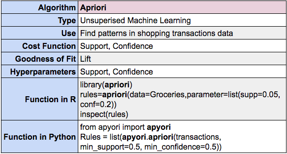
This algorithm calculates the support, confidence, and lift for all possible combination of products which satisfies a minimum threshold of support and confidence. Hence, reducing the computation required. Otherwise, there will be too many combinations.
This activity is performed in two major steps:
- Find out the frequent combination of items called “itemsets” which satisfy the minimum support threshold.
- Generate association from frequent itemsets rules based on the minimum confidence threshold.
The above style of finding association rules is based on the breadth-first search strategy, hence, it needs to scan the database multiple times. Due to this, the Apriori algorithm is slow. It is often criticized for not being able to handle very large datasets efficiently.
Apriori algorithm calculates the support, confidence, and lift for all possible combination of products which satisfies a minimum threshold of support and confidence.
Step-1: Finding the frequent itemsets: It is an iterative process, with pruning involved in each step.
We start with one item at a time and keep increasing the items in the itemset.
- items=1, start finding itemsets of one product each. Compute the support for each itemset and remove those which does not satisfy the minimum support threshold.
- items=2, start finding combinations of 2 products as an itemset. Compute the support for each itemset and remove those which does not satisfy the minimum support threshold.
- items=3, start finding combinations of 3 products as an itemset. Compute the support for each itemset and remove those which does not satisfy the minimum support threshold.
- keep repeating the process until maximum possible combinations are covered.
Step-2: Creating rules from itemsets: It is an iterative process, with elimination involved in each step.
Example: If an itemset contains 4 elements {Milk, Bread, Cold Drink, Wafer} then follow the below steps by starting with only one item in the RHS and keep decreasing the elements in LHS to formulate and evaluate new rules.
- Find the confidence of rule {Milk,Bread,Cold Drink -> Wafer}, if it is more than the minimum confidence threshold then keep it otherwise reject.
- Find the confidence of rule {Milk,Bread -> Cold Drink,Wafer}, if it is more than the minimum confidence threshold then keep it otherwise reject.
- Find the confidence of rule {Milk -> Bread,Cold Drink,Wafer}, if it is more than the minimum confidence threshold then keep it otherwise reject.
- Find the confidence of rule {Bread,Cold Drink,Wafer -> Milk}, if it is more than the minimum confidence threshold then keep it otherwise reject.
- Find the confidence of rule {Bread,Cold Drink -> Wafer,Milk}, if it is more than the minimum confidence threshold then keep it otherwise reject.
- Find the confidence of rule {Bread -> Cold Drink,Wafer,Milk}, if it is more than the minimum confidence threshold then keep it otherwise reject.
So on and so forth… The above steps are repeated for each and every itemsets found with minimum support and confidence level.
In the end, we are left with those rules which satisfy the minimum support and confidence threshold.
Q. How to run Apriori in R?
|
1 2 3 4 5 6 7 8 9 10 11 12 13 14 15 16 17 18 19 |
# Sample code to do Apriori in R # Loading a sample transactions data # If you want to create this class of data set using a csv/data.frame then use transactions() function data("Groceries") inspect(Groceries[1:10]) # Find itemsets with min support threshold of 0.5 and min confidence of 0.2 # Smaller values of Support and confidence threshold will generate more rules library(apriori) rules=apriori(data=Groceries,parameter=list(supp=0.05, conf=0.2)) inspect(rules) # Sorting rules by confidence SortedRules=sort(rules, by='confidence') inspect(SortedRules) # Sorting rules by lift SortedRules=sort(rules, by='lift') inspect(SortedRules) |
Q. How to run Apriori in Python?
|
1 2 3 4 5 6 7 8 9 10 11 12 13 14 15 16 17 18 19 20 21 22 23 24 25 26 27 28 29 |
# Library installtion for apriori # !pip install apyori # Sample code to do Apriori in Python import apyori # Creating Sample Transactions transactions = [ ['Milk', 'Bread', 'Saffron'], ['Milk', 'Saffron'], ['Bread', 'Saffron','Wafer'], ['Bread','Wafer'], ] # Generating association rules Rules = list(apyori.apriori(transactions, min_support=0.5, min_confidence=0.5)) # Extracting rules from the object for i in range(len(Rules)): LHS=list(Rules[i][2][0][0]) RHS=list(Rules[i][2][0][1]) support=Rules[i][1] confidence=Rules[i][2][0][2] lift=Rules[i][2][0][3] print("LHS:",LHS,"--","RHS:",RHS) print("Support:",support) print("Confidence:",confidence) print("Lift:",lift) print(10*"----") |
Q How does the Eclat algorithm work?

ECLAT stands for Equivalence CLAss Transformation! The basic idea is the same as the apriori algorithm but the ECLAT algorithm addresses and improves two major issues in apriori.
- ECLAT uses Depth First Search while scanning the transactions database, this is done by defining a “vertical database” which is based on “tid-list” which is nothing but a list of transactions where an itemset(a combination of items) was purchased together.
- This approach reduces the number of database scans needed to find all the rules. Hence We can use ECLAT on large databases.
- ECLAT uses the “lattice-theoric” approach. It breaks down the largest combination of items(biggest lattice) into smaller subsets(sublattices) and processes each smaller subsets to find association rules. Hence can be executed in parallel and reduces the time taken.
- Eclat uses any one of the bottom-up approach / top-down approach/hybrid search approaches to find sublattices.
ECLAT generates association rules in two major steps which are the same as used in apriori.
- Find out the frequent combination of items called “itemsets” which satisfy the minimum support threshold.
- Generate association rules from frequent itemsets based on the minimum confidence threshold.
The Key difference is HOW ECLAT finds the frequent “itemsets”? Here ECLAT is more efficient than apriori.
The Key difference is HOW ECLAT finds the frequent “itemsets”? Here ECLAT is more efficient than apriori.
Step-1: Find out the frequent combination of items called “itemsets”
- This begins by finding those combinations of items (itemsets) which contains the maximum number of items among all other itemsets and has the maximum frequency in the transactions database. These are known as “maximal frequent itemsets”.
- All other itemsets are subsets of these itemsets. Hence these are the starting points (Starting Big Lattice).
- Keep making smaller combinations of itemsets from “maximal frequent itemsets”
- Example: If a maximal frequent itemset has 4 items {Milk,Bread,Cold Drink,Wafer} then the algorithm will start creating smaller subsets which satisfies minimum support threshold e.g. {Milk,Bread,Cold Drink}, {Milk,Bread,Wafer}, {Bread,Cold Drink,Wafer},{Milk,Bread}, {Milk}etc.
Step-2: Generate Association rules using the minimum confidence threshold.
- For each of the itemsets calculate the confidence and keep eliminating those rules which do not satisfy the minimum confidence threshold.
- Example: If an itemset contains 4 elements {Milk, Bread, Cold Drink, Wafer} then follow the below steps by starting with only one item in the RHS and keep decreasing the elements in LHS to formulate and evaluate new rules.
- Find the confidence of rule {Milk,Bread,Cold Drink -> Wafer}, if it is more than the minimum confidence threshold then keep it otherwise reject.
- Find the confidence of rule {Milk,Bread -> Cold Drink,Wafer}, if it is more than the minimum confidence threshold then keep it otherwise reject.
- Find the confidence of rule {Milk -> Bread,Cold Drink,Wafer}, if it is more than the minimum confidence threshold then keep it otherwise reject.
- Find the confidence of rule {Bread,Cold Drink,Wafer -> Milk}, if it is more than the minimum confidence threshold then keep it otherwise reject.
- Find the confidence of rule {Bread,Cold Drink -> Wafer,Milk}, if it is more than the minimum confidence threshold then keep it otherwise reject.
- Find the confidence of rule {Bread -> Cold Drink,Wafer,Milk}, if it is more than the minimum confidence threshold then keep it otherwise reject.
- So on and so forth…
The above steps are repeated for each and every itemsets found with minimum support and confidence level.
In the end, we are left with those rules which satisfy the minimum support and confidence threshold.
Q. How to run Eclat in R?
|
1 2 3 4 5 6 7 8 9 10 11 12 13 14 15 16 17 18 19 20 21 22 23 24 |
# Sample code to do Eclat in R # Loading a sample transactions data # If you want to create this class of data set using a csv/data.frame then use transactions() function data("Groceries") inspect(Groceries[1:10]) # Find itemsets with minimum support threshold of 0.5 and 5 or less items # Smaller values of Support threshold will generate more itemsets library(apriori) FrequentItemsets=eclat(data=Groceries,parameter=list(supp=0.05, maxlen=5)) inspect(FrequentItemsets) # Create rules from the itemsets with minimum confidence threshold of 0.2 rules=ruleInduction(x=FrequentItemsets, transactions=Groceries, confidence = 0.2) inspect(rules) # Sorting rules by confidence SortedRules=sort(rules, by='confidence') inspect(SortedRules) # Sorting rules by lift SortedRules=sort(rules, by='lift') inspect(SortedRules) |
Q. How to run Eclat in Python?
|
1 2 3 4 5 6 7 8 9 10 11 12 13 14 15 16 17 |
# Sample code to do Eclat in Python # The package source can be found at below location, it is not stable however # https://github.com/andi611/Apriori-and-Eclat-Frequent-Itemset-Mining from association import eclat # Creating Sample Transactions transactions = [ ['Milk', 'Bread', 'Saffron'], ['Milk', 'Saffron'], ['Bread', 'Saffron','Wafer'], ['Bread','Wafer'], ] # Creating Rules using Eclat Rules=eclat.eclat(data=transactions, min_support=0.5) Rules |
Q How does the FP-Growth algorithm work?

FP-Growth stands for Frequent Patterns Growth. This algorithm is faster than apriori but not suitable for large datasets due to high memory requirements.
Like Apriori and ECLAT, FP-Growth also generates rules in two steps:
- Find out the frequent combination of items called “itemsets” which satisfy the minimum support threshold.
- Generate association rules from frequent itemsets based on the minimum confidence threshold.
The main difference between apriori and FP-Growth is the way FP-Growth FINDS frequent itemsets.
FP-Growth algorithm uses a special tree data structure known as “FP-Tree” that stores the frequent patterns at one place
This tree helps to reduce the need for scanning databases dramatically! In only two scans, all the frequent itemsets are found.
Once all the frequent itemsets are found, then the rules are generated using the tree.
FP-Growth algorithm uses a special tree data structure known as “FP-Tree” that stores the frequent patterns at one place
This tree helps to reduce the need for scanning databases dramatically! In only two scans, all the frequent itemsets are found.
Let’s examine how FP-Growth works using below sample transactions dataset:
Step-1. Find out the frequent combination of items called “itemsets”
1. Find out the support of every item in the transactions dataset and arrange them in decreasing order, if two items have the same support then arrange them alphabetically.

Choose only those items which are above a minimum support threshold.
for example: {Milk:4, Cold Drink:3, Bread:2, Wafer:2, Saffron:1}
Now if the minimum threshold=2 is applied, then Saffron will get eliminated and we will get only
{Milk:4, Cold Drink:3, Bread:2, Wafer:2}
This simple elimination reduces a lot of computing effort! We will now construct the FP-Tree for only those remaining items.

2. Arrange the items present in every transaction in decreasing order of support
For example, {Cold Drink, Milk, Wafer} will be arranged like {Milk:4, Cold Drink:3, Wafer:2}
Milk gets the first position because it has maximum support and Wafer gets the last position since it has the least support value.
3. Create the FP-Tree by inserting one transaction at a time
- Transaction-1: Milk:4 gets inserted and frequency incremented by 1
- Transaction-2: Milk:4, Bread:2 gets inserted, and frequency incremented by 1, hence, Milk has frequency=2 and others has frequency=1
- Transaction-3: Milk:4, Bread:2 gets inserted and frequency is incremented by 1, hence, Milk has frequency 3 now and Bread has frequency=2
- Transaction-4: Cold Drink:3, Wafer:2 gets inserted. This creates a new leg from the root, with frequency as 1 for both items
- Transaction-5: Cold Drink:3 gets inserted in the same leg, the frequency is updated as 2
- Transaction-6: Milk:4, Cold Drink:3, Wafer:2 gets inserted, the frequency is incremented by 1.
4. Read the FP-Tree to find the path(known as a prefix) of each item.
This helps to count the number of ways to reach an item in the tree.
To reach Bread, we have one way possible but it is repeated 2 times in the transactions. Milk->Bread
To reach Milk we start from the root node hence, it is an empty path.

5. Generate Frequent itemsets
Combine the item with its path and make sure all combinations are taken into account
For example: if We are reaching to Saffron via Milk->Bread, then the frequent itemsets will be
{Saffron,Milk}, {Saffron,Bread}, {Milk,Saffron,Bread}
Step-2: Generate Association rules using the minimum confidence threshold.
1. For each of the itemsets calculate the confidence and keep eliminating those rules which do not satisfy the minimum confidence threshold.
Example: If an itemset contains 4 elements {Milk, Bread, Cold Drink, Wafer} then follow below steps by starting with only one item
In the RHS and keep decreasing the elements in LHS to formulate and evaluate new rules.
- Find the confidence of rule {Milk,Bread,Cold Drink -> Wafer}, if it is more than the minimum confidence threshold then keep it otherwise reject.
- Find the confidence of rule {Milk,Bread -> Cold Drink,Wafer}, if it is more than the minimum confidence threshold then keep it otherwise reject.
- Find the confidence of rule {Milk -> Bread,Cold Drink,Wafer}, if it is more than the minimum confidence threshold then keep it otherwise reject.
- Find the confidence of rule {Bread,Cold Drink,Wafer -> Milk}, if it is more than the minimum confidence threshold then keep it otherwise reject.
- Find the confidence of rule {Bread,Cold Drink -> Wafer,Milk}, if it is more than the minimum confidence threshold then keep it otherwise reject.
- Find the confidence of rule {Bread -> Cold Drink,Wafer,Milk}, if it is more than the minimum confidence threshold then keep it otherwise reject.
- So on and so forth…
The above steps are repeated for each and every itemsets found with minimum support and confidence level.
In the end, we are left with those rules which satisfy the minimum support and confidence threshold.
Q. How to run FP-Growth in R?
|
1 2 3 4 5 6 7 8 9 10 11 12 13 14 15 16 17 18 19 20 21 |
# Sample code to do FP-Growth in R # Loading a sample transactions data # If you want to create this class of data set using a csv/data.frame then use transactions() function data("Groceries") inspect(Groceries[1:10]) # Find itemsets with and 5 or less items # Smaller values of Support threshold will generate more itemsets library(rCBA) # Create rules from the itemsets with minimum support threshold of 0.5 and minimum confidence threshold of 0.2 rules=rCBA::fpgrowth(Groceries, support=0.5, confidence=0.2,maxLength=2,consequent="other vegetables") inspect(rules) # Sorting rules by confidence SortedRules=sort(rules, by='confidence') inspect(SortedRules) # Sorting rules by lift SortedRules=sort(rules, by='lift') inspect(SortedRules) |
Q. How to run FP-Growth in Python?
|
1 2 3 4 5 6 7 8 9 10 11 12 13 14 15 16 17 |
# Sample code to do FP-Growth in Python import pyfpgrowth # Creating Sample Transactions transactions = [ ['Milk', 'Bread', 'Saffron'], ['Milk', 'Saffron'], ['Bread', 'Saffron','Wafer'], ['Bread','Wafer'], ] #Finding the frequent patterns with min support threshold=0.5 FrequentPatterns=pyfpgrowth.find_frequent_patterns(transactions=transactions,support_threshold=0.5) print(FrequentPatterns) # Generating rules with min confidence threshold=0.5 Rules=pyfpgrowth.generate_association_rules(patterns=FrequentPatterns,confidence_threshold=0.5) Rules |
Conclusion
In this post I have explained some of the important algorithms used for Unsupervised ML, with these, you will be able to solve a wide variety of problems falling under Unsupervised ML.
There are many more algorithms which you can explore further here!
Let me know in case you want an explanation for any other Unsupervised ML algorithm. I will include it in this post.
In the next post, I will talk about the interview questions related to reinforced machine learning.
All the best for that interview!